A violin plot is a compact display of a continuous distribution. It is a
blend of geom_boxplot() and geom_density(): a
violin plot is a mirrored density plot displayed in the same way as a
boxplot.
Usage
geom_violin(
  mapping = NULL,
  data = NULL,
  stat = "ydensity",
  position = "dodge",
  ...,
  trim = TRUE,
  bounds = c(-Inf, Inf),
  quantile.colour = NULL,
  quantile.color = NULL,
  quantile.linetype = 0L,
  quantile.linewidth = NULL,
  draw_quantiles = deprecated(),
  scale = "area",
  na.rm = FALSE,
  orientation = NA,
  show.legend = NA,
  inherit.aes = TRUE
)

stat_ydensity(
  mapping = NULL,
  data = NULL,
  geom = "violin",
  position = "dodge",
  ...,
  orientation = NA,
  bw = "nrd0",
  adjust = 1,
  kernel = "gaussian",
  trim = TRUE,
  scale = "area",
  drop = TRUE,
  bounds = c(-Inf, Inf),
  quantiles = c(0.25, 0.5, 0.75),
  na.rm = FALSE,
  show.legend = NA,
  inherit.aes = TRUE
)
Arguments
- mapping
Set of aesthetic mappings created by
aes(). If specified andinherit.aes = TRUE(the default), it is combined with the default mapping at the top level of the plot. You must supplymappingif there is no plot mapping.- data
The data to be displayed in this layer. There are three options:
If
NULL, the default, the data is inherited from the plot data as specified in the call toggplot().A
data.frame, or other object, will override the plot data. All objects will be fortified to produce a data frame. Seefortify()for which variables will be created.A
functionwill be called with a single argument, the plot data. The return value must be adata.frame, and will be used as the layer data. Afunctioncan be created from aformula(e.g.~ head(.x, 10)).- position
A position adjustment to use on the data for this layer. This can be used in various ways, including to prevent overplotting and improving the display. The
positionargument accepts the following:The result of calling a position function, such as
position_jitter(). This method allows for passing extra arguments to the position.A string naming the position adjustment. To give the position as a string, strip the function name of the
position_prefix. For example, to useposition_jitter(), give the position as"jitter".For more information and other ways to specify the position, see the layer position documentation.
- ...
Other arguments passed on to
layer()'sparamsargument. These arguments broadly fall into one of 4 categories below. Notably, further arguments to thepositionargument, or aesthetics that are required can not be passed through.... Unknown arguments that are not part of the 4 categories below are ignored.Static aesthetics that are not mapped to a scale, but are at a fixed value and apply to the layer as a whole. For example,
colour = "red"orlinewidth = 3. The geom's documentation has an Aesthetics section that lists the available options. The 'required' aesthetics cannot be passed on to theparams. Please note that while passing unmapped aesthetics as vectors is technically possible, the order and required length is not guaranteed to be parallel to the input data.When constructing a layer using a
stat_*()function, the...argument can be used to pass on parameters to thegeompart of the layer. An example of this isstat_density(geom = "area", outline.type = "both"). The geom's documentation lists which parameters it can accept.Inversely, when constructing a layer using a
geom_*()function, the...argument can be used to pass on parameters to thestatpart of the layer. An example of this isgeom_area(stat = "density", adjust = 0.5). The stat's documentation lists which parameters it can accept.The
key_glyphargument oflayer()may also be passed on through.... This can be one of the functions described as key glyphs, to change the display of the layer in the legend.
- trim
If
TRUE(default), trim the tails of the violins to the range of the data. IfFALSE, don't trim the tails.- bounds
Known lower and upper bounds for estimated data. Default
c(-Inf, Inf)means that there are no (finite) bounds. If any bound is finite, boundary effect of default density estimation will be corrected by reflecting tails outsideboundsaround their closest edge. Data points outside of bounds are removed with a warning.- quantile.colour, quantile.color, quantile.linewidth, quantile.linetype
Default aesthetics for the quantile lines. Set to
NULLto inherit from the data's aesthetics. By default, quantile lines are hidden and can be turned on by changingquantile.linetype. Quantile values can be set using thequantilesargument when usingstat = "ydensity"(default).- draw_quantiles
![[Deprecated]](figures/lifecycle-deprecated.svg) Previous
specification of drawing quantiles.
Previous
specification of drawing quantiles.- scale
if "area" (default), all violins have the same area (before trimming the tails). If "count", areas are scaled proportionally to the number of observations. If "width", all violins have the same maximum width.
- na.rm
If
FALSE, the default, missing values are removed with a warning. IfTRUE, missing values are silently removed.- orientation
The orientation of the layer. The default (
NA) automatically determines the orientation from the aesthetic mapping. In the rare event that this fails it can be given explicitly by settingorientationto either"x"or"y". See the Orientation section for more detail.- show.legend
logical. Should this layer be included in the legends?
NA, the default, includes if any aesthetics are mapped.FALSEnever includes, andTRUEalways includes. It can also be a named logical vector to finely select the aesthetics to display. To include legend keys for all levels, even when no data exists, useTRUE. IfNA, all levels are shown in legend, but unobserved levels are omitted.- inherit.aes
If
FALSE, overrides the default aesthetics, rather than combining with them. This is most useful for helper functions that define both data and aesthetics and shouldn't inherit behaviour from the default plot specification, e.g.annotation_borders().- geom, stat
Use to override the default connection between
geom_violin()andstat_ydensity(). For more information about overriding these connections, see how the stat and geom arguments work.- bw
The smoothing bandwidth to be used. If numeric, the standard deviation of the smoothing kernel. If character, a rule to choose the bandwidth, as listed in
stats::bw.nrd(). Note that automatic calculation of the bandwidth does not take weights into account.- adjust
A multiplicate bandwidth adjustment. This makes it possible to adjust the bandwidth while still using the a bandwidth estimator. For example,
adjust = 1/2means use half of the default bandwidth.- kernel
Kernel. See list of available kernels in
density().- drop
Whether to discard groups with less than 2 observations (
TRUE, default) or keep such groups for position adjustment purposes (FALSE).- quantiles
A numeric vector with numbers between 0 and 1 to indicate quantiles marked by the
quantilecomputed variable. The default marks the 25th, 50th and 75th percentiles. The display of quantiles can be turned on by settingquantile.linetypeto non-blank when usinggeom = "violin"(default).
Orientation
This geom treats each axis differently and, thus, can thus have two orientations. Often the orientation is easy to deduce from a combination of the given mappings and the types of positional scales in use. Thus, ggplot2 will by default try to guess which orientation the layer should have. Under rare circumstances, the orientation is ambiguous and guessing may fail. In that case the orientation can be specified directly using the orientation parameter, which can be either "x" or "y". The value gives the axis that the geom should run along, "x" being the default orientation you would expect for the geom.
Computed variables
These are calculated by the 'stat' part of layers and can be accessed with delayed evaluation.
after_stat(density)
Density estimate.after_stat(scaled)
Density estimate, scaled to a maximum of 1.after_stat(count)
Density * number of points - probably useless for violin plots.after_stat(violinwidth)
Density scaled for the violin plot, according to area, counts or to a constant maximum width.after_stat(n)
Number of points.after_stat(width)
Width of violin bounding box.after_stat(quantile)
Whether the row is part of thequantilescomputation.
References
Hintze, J. L., Nelson, R. D. (1998) Violin Plots: A Box Plot-Density Trace Synergism. The American Statistician 52, 181-184.
See also
geom_violin() for examples, and stat_density()
for examples with data along the x axis.
Aesthetics
geom_violin() understands the following aesthetics. Required aesthetics are displayed in bold and defaults are displayed for optional aesthetics:
| • | x | |
| • | y | |
| • | alpha | → NA |
| • | colour | → via theme() |
| • | fill | → via theme() |
| • | group | → inferred |
| • | linetype | → via theme() |
| • | linewidth | → via theme() |
| • | weight | → 1 |
| • | width | → 0.9 |
Learn more about setting these aesthetics in vignette("ggplot2-specs").
Examples
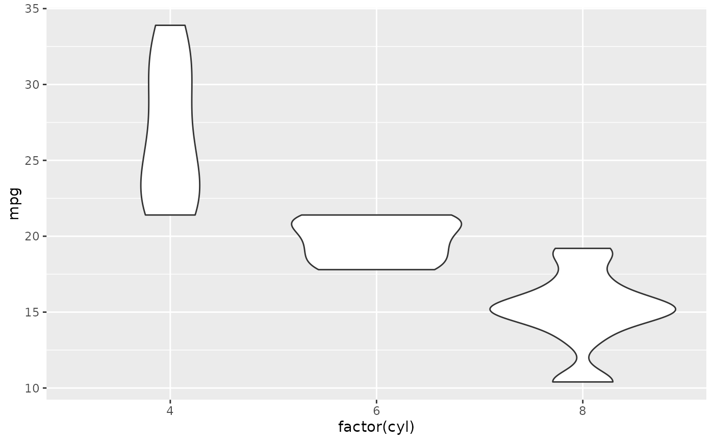
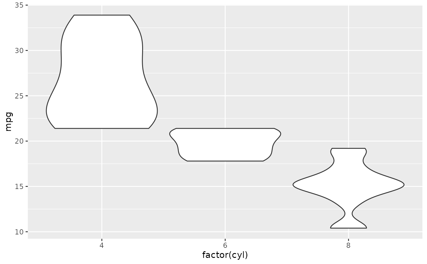
p <- ggplot(mtcars, aes(factor(cyl), mpg))
p + geom_violin()
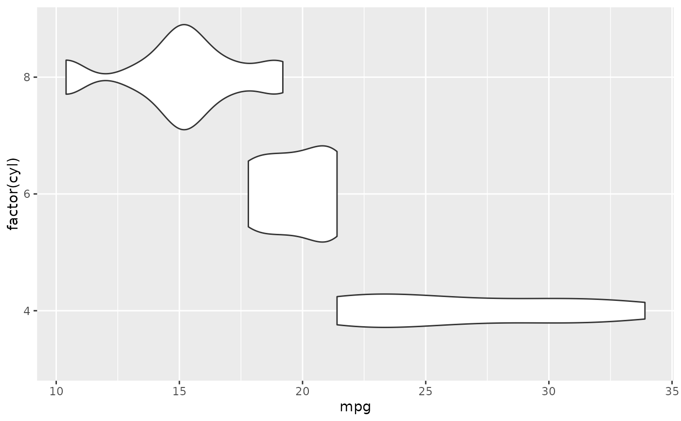
 # Orientation follows the discrete axis
ggplot(mtcars, aes(mpg, factor(cyl))) +
geom_violin()
# Orientation follows the discrete axis
ggplot(mtcars, aes(mpg, factor(cyl))) +
geom_violin()
 # \donttest{
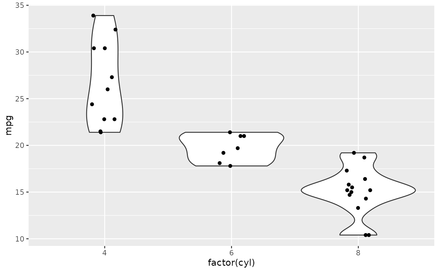
p + geom_violin() + geom_jitter(height = 0, width = 0.1)
# \donttest{
p + geom_violin() + geom_jitter(height = 0, width = 0.1)
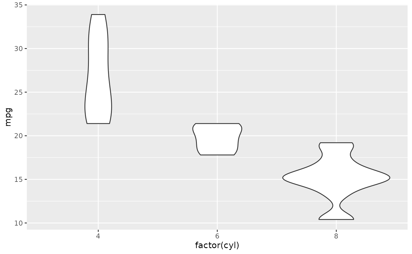
 # Scale maximum width proportional to sample size:
p + geom_violin(scale = "count")
# Scale maximum width proportional to sample size:
p + geom_violin(scale = "count")
 # Scale maximum width to 1 for all violins:
p + geom_violin(scale = "width")
# Scale maximum width to 1 for all violins:
p + geom_violin(scale = "width")
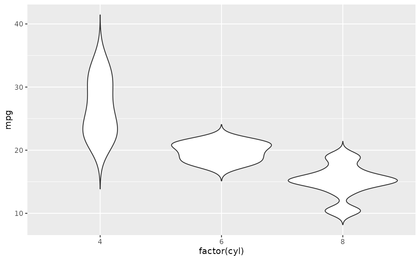
 # Default is to trim violins to the range of the data. To disable:
p + geom_violin(trim = FALSE)
# Default is to trim violins to the range of the data. To disable:
p + geom_violin(trim = FALSE)
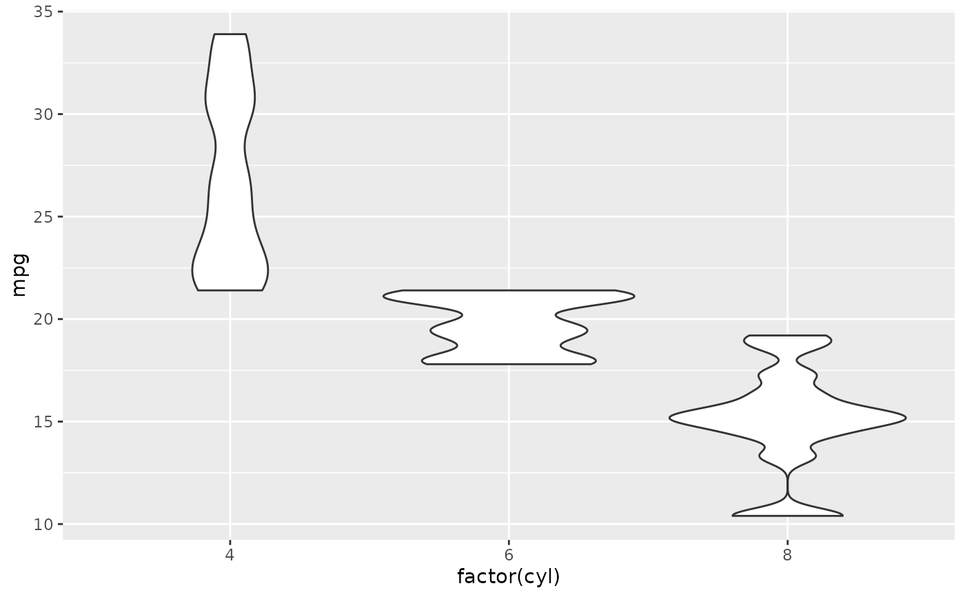
 # Use a smaller bandwidth for closer density fit (default is 1).
p + geom_violin(adjust = .5)
# Use a smaller bandwidth for closer density fit (default is 1).
p + geom_violin(adjust = .5)
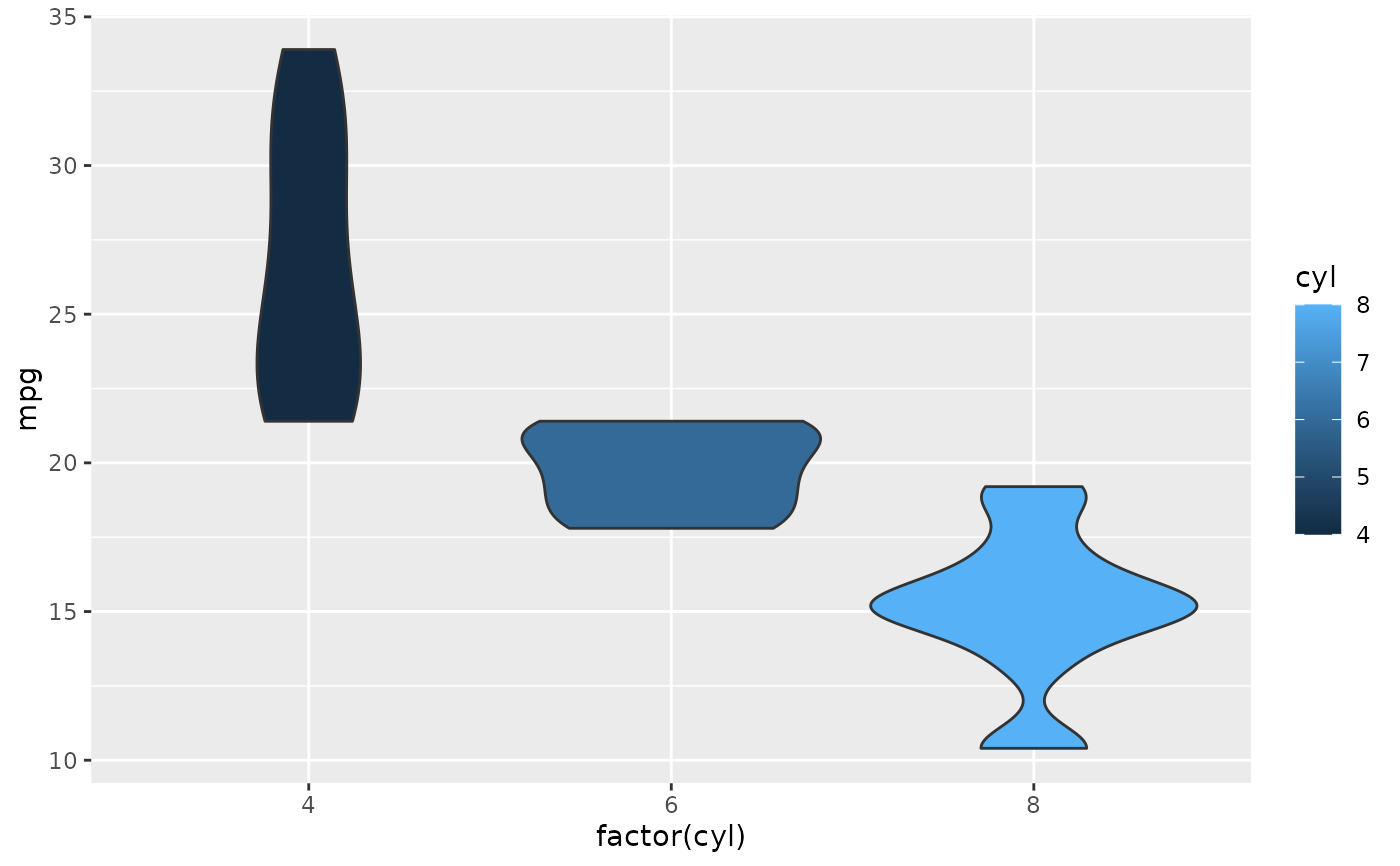
 # Add aesthetic mappings
# Note that violins are automatically dodged when any aesthetic is
# a factor
p + geom_violin(aes(fill = cyl))
# Add aesthetic mappings
# Note that violins are automatically dodged when any aesthetic is
# a factor
p + geom_violin(aes(fill = cyl))
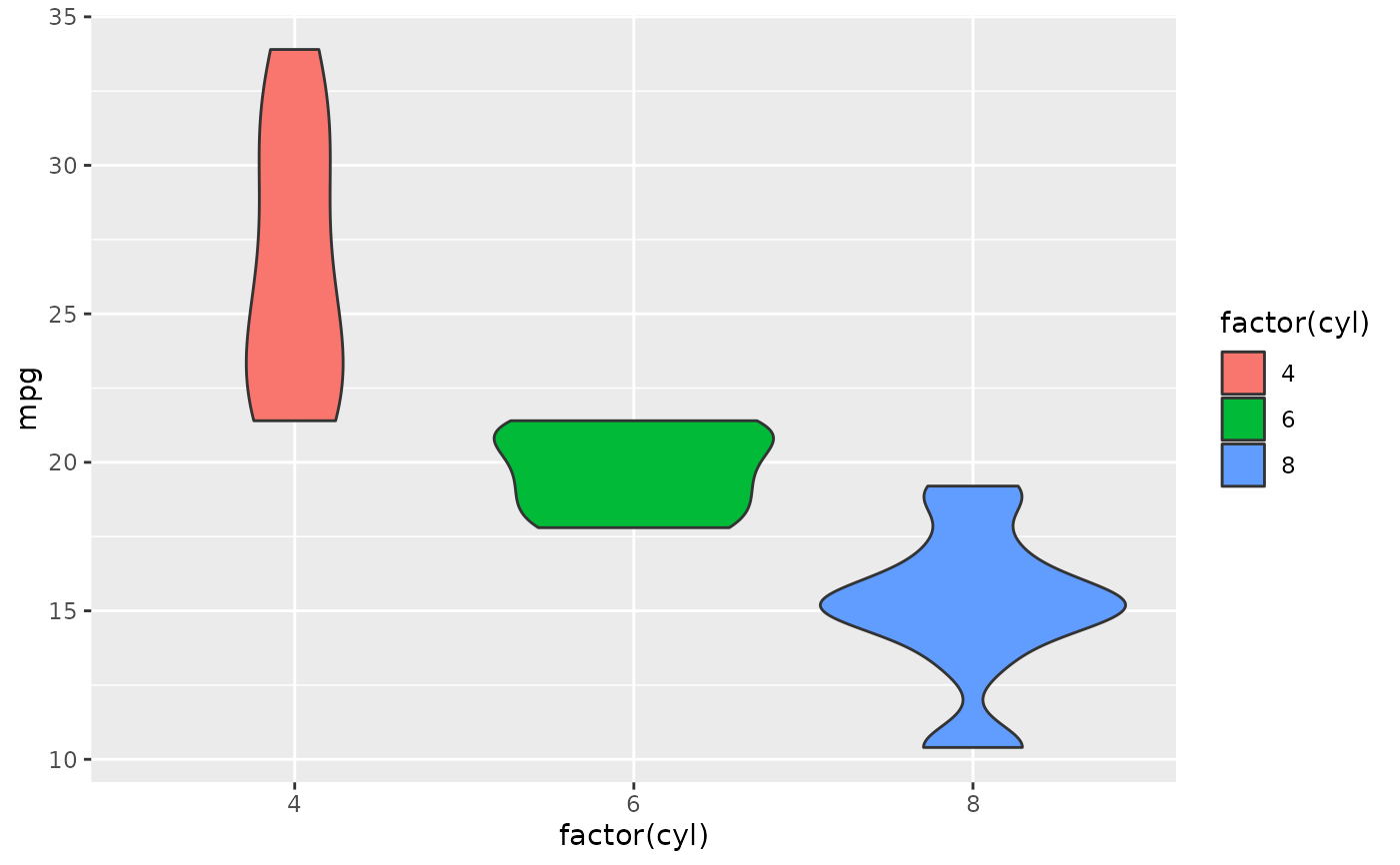
 p + geom_violin(aes(fill = factor(cyl)))
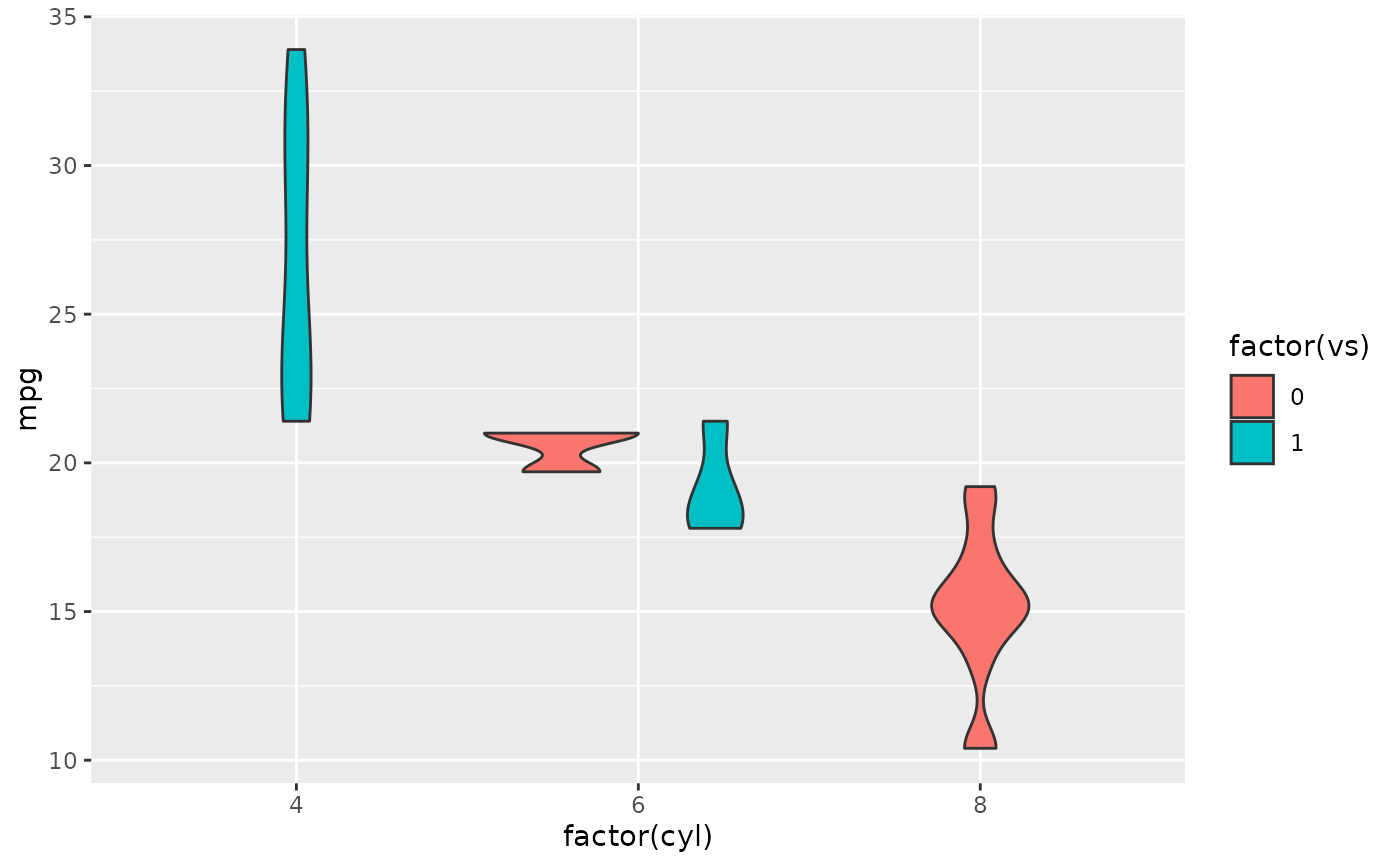
 p + geom_violin(aes(fill = factor(vs)))
#> Warning: Groups with fewer than two datapoints have been dropped.
#> ℹ Set `drop = FALSE` to consider such groups for position adjustment
#> purposes.
p + geom_violin(aes(fill = factor(vs)))
#> Warning: Groups with fewer than two datapoints have been dropped.
#> ℹ Set `drop = FALSE` to consider such groups for position adjustment
#> purposes.
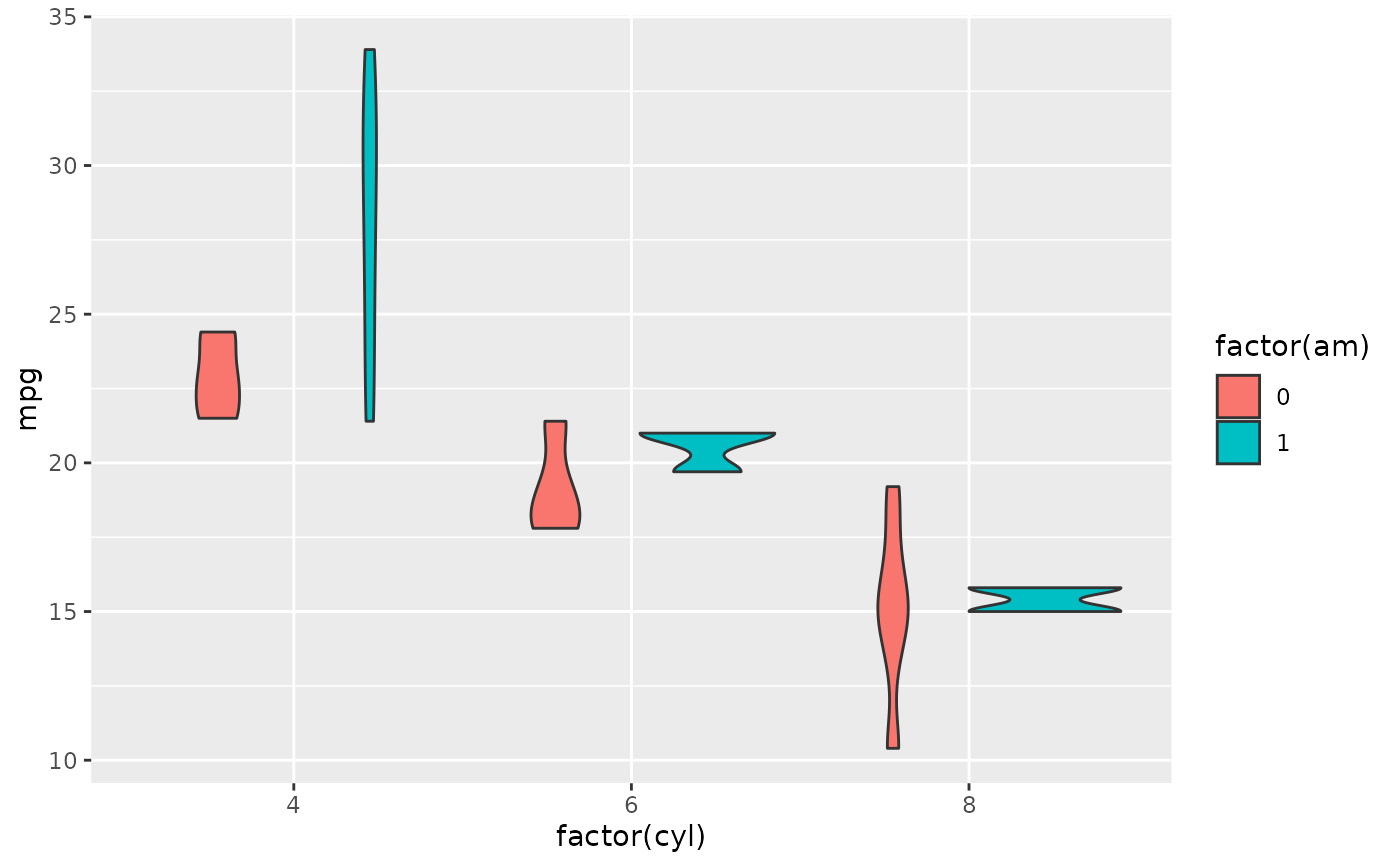
 p + geom_violin(aes(fill = factor(am)))
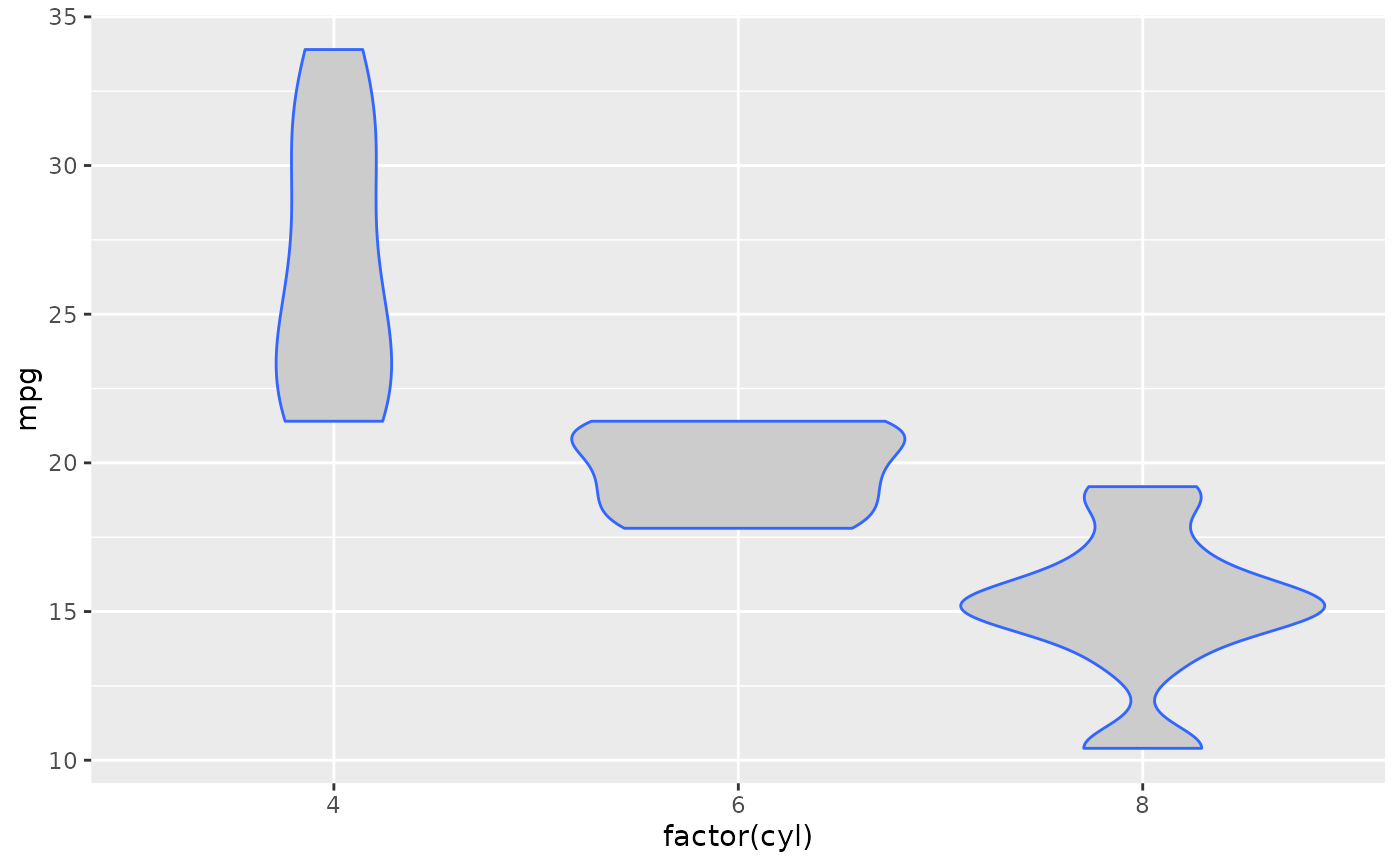
 # Set aesthetics to fixed value
p + geom_violin(fill = "grey80", colour = "#3366FF")
# Set aesthetics to fixed value
p + geom_violin(fill = "grey80", colour = "#3366FF")
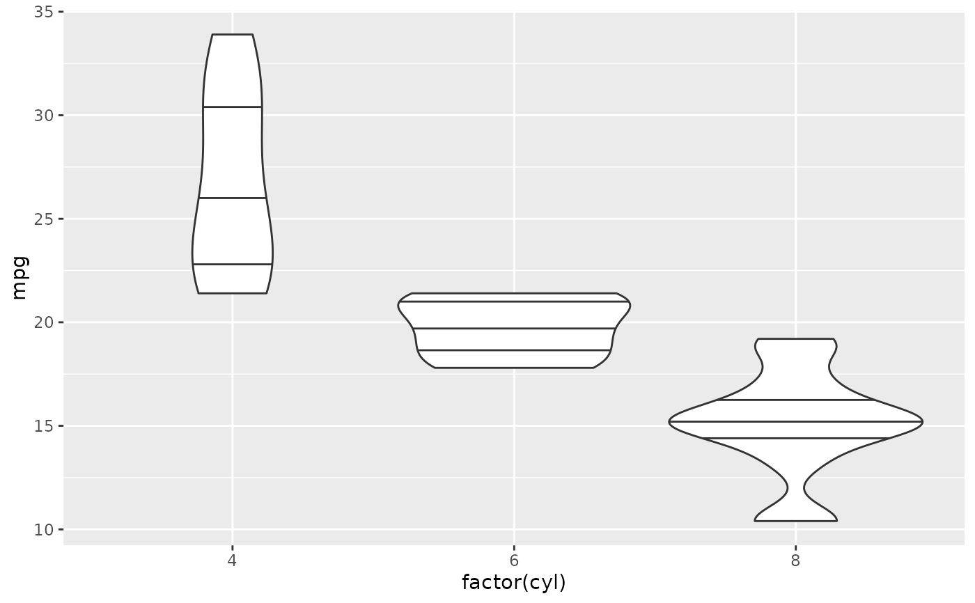
 # Show quartiles
p + geom_violin(draw_quantiles = c(0.25, 0.5, 0.75))
#> Warning: The `draw_quantiles` argument of `geom_violin()` is deprecated as of
#> ggplot2 4.0.0.
#> ℹ Please use the `quantiles.linetype` argument instead.
# Show quartiles
p + geom_violin(draw_quantiles = c(0.25, 0.5, 0.75))
#> Warning: The `draw_quantiles` argument of `geom_violin()` is deprecated as of
#> ggplot2 4.0.0.
#> ℹ Please use the `quantiles.linetype` argument instead.
 # Scales vs. coordinate transforms -------
if (require("ggplot2movies")) {
# Scale transformations occur before the density statistics are computed.
# Coordinate transformations occur afterwards. Observe the effect on the
# number of outliers.
m <- ggplot(movies, aes(y = votes, x = rating, group = cut_width(rating, 0.5)))
m + geom_violin()
m +
geom_violin() +
scale_y_log10()
m +
geom_violin() +
coord_transform(y = "log10")
m +
geom_violin() +
scale_y_log10() + coord_transform(y = "log10")
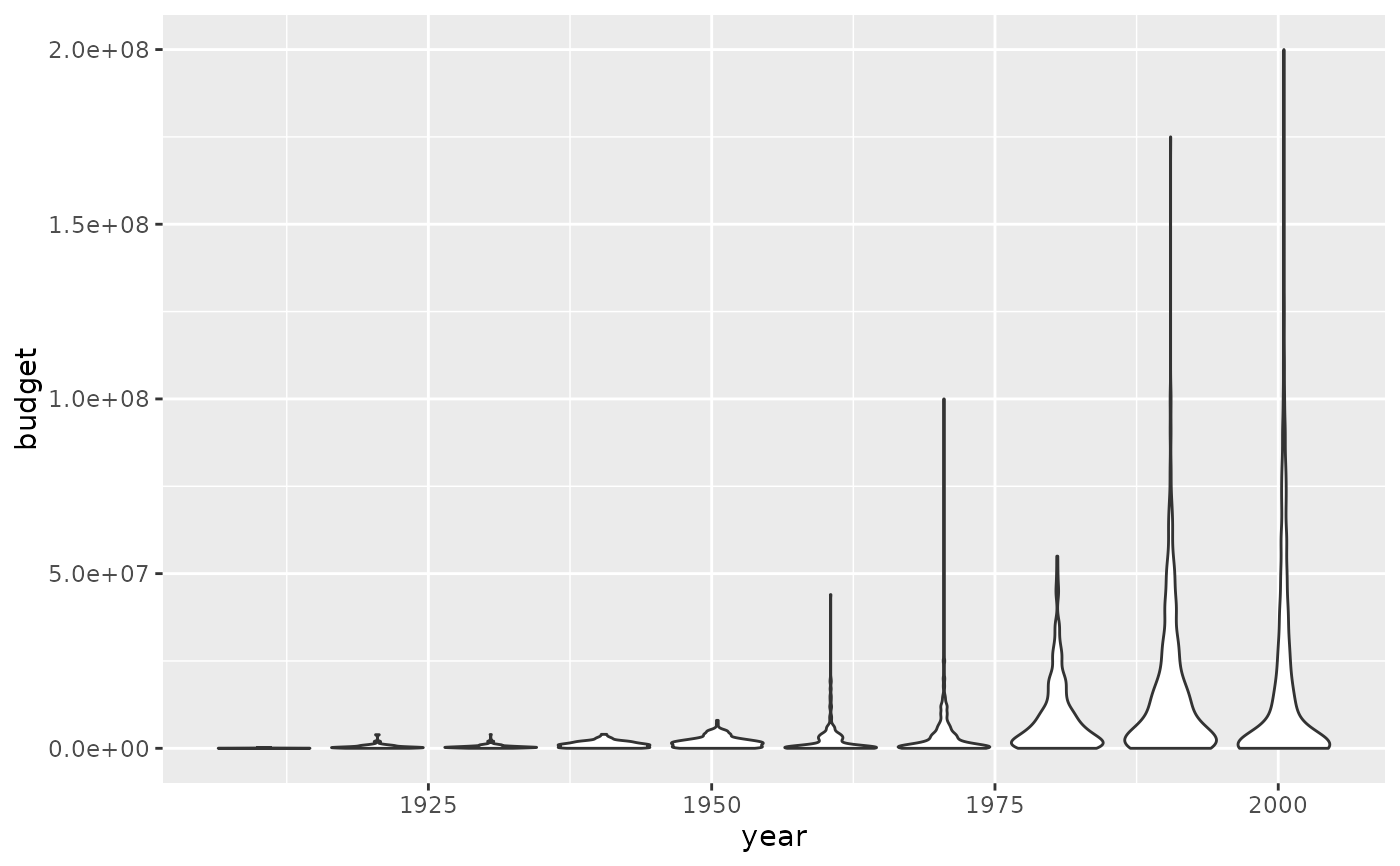
# Violin plots with continuous x:
# Use the group aesthetic to group observations in violins
ggplot(movies, aes(year, budget)) +
geom_violin()
ggplot(movies, aes(year, budget)) +
geom_violin(aes(group = cut_width(year, 10)), scale = "width")
}
#> Warning: Removed 53573 rows containing non-finite outside the scale range
#> (`stat_ydensity()`).
#> Warning: Groups with fewer than two datapoints have been dropped.
#> ℹ Set `drop = FALSE` to consider such groups for position adjustment
#> purposes.
# Scales vs. coordinate transforms -------
if (require("ggplot2movies")) {
# Scale transformations occur before the density statistics are computed.
# Coordinate transformations occur afterwards. Observe the effect on the
# number of outliers.
m <- ggplot(movies, aes(y = votes, x = rating, group = cut_width(rating, 0.5)))
m + geom_violin()
m +
geom_violin() +
scale_y_log10()
m +
geom_violin() +
coord_transform(y = "log10")
m +
geom_violin() +
scale_y_log10() + coord_transform(y = "log10")
# Violin plots with continuous x:
# Use the group aesthetic to group observations in violins
ggplot(movies, aes(year, budget)) +
geom_violin()
ggplot(movies, aes(year, budget)) +
geom_violin(aes(group = cut_width(year, 10)), scale = "width")
}
#> Warning: Removed 53573 rows containing non-finite outside the scale range
#> (`stat_ydensity()`).
#> Warning: Groups with fewer than two datapoints have been dropped.
#> ℹ Set `drop = FALSE` to consider such groups for position adjustment
#> purposes.
 # }
# }