Computes and draws kernel density estimate, which is a smoothed version of the histogram. This is a useful alternative to the histogram for continuous data that comes from an underlying smooth distribution.
Usage
geom_density(
  mapping = NULL,
  data = NULL,
  stat = "density",
  position = "identity",
  ...,
  outline.type = "upper",
  lineend = "butt",
  linejoin = "round",
  linemitre = 10,
  na.rm = FALSE,
  show.legend = NA,
  inherit.aes = TRUE
)

stat_density(
  mapping = NULL,
  data = NULL,
  geom = "area",
  position = "stack",
  ...,
  orientation = NA,
  bw = "nrd0",
  adjust = 1,
  kernel = "gaussian",
  n = 512,
  trim = FALSE,
  bounds = c(-Inf, Inf),
  na.rm = FALSE,
  show.legend = NA,
  inherit.aes = TRUE
)
Arguments
- mapping
Set of aesthetic mappings created by
aes(). If specified andinherit.aes = TRUE(the default), it is combined with the default mapping at the top level of the plot. You must supplymappingif there is no plot mapping.- data
The data to be displayed in this layer. There are three options:
If
NULL, the default, the data is inherited from the plot data as specified in the call toggplot().A
data.frame, or other object, will override the plot data. All objects will be fortified to produce a data frame. Seefortify()for which variables will be created.A
functionwill be called with a single argument, the plot data. The return value must be adata.frame, and will be used as the layer data. Afunctioncan be created from aformula(e.g.~ head(.x, 10)).- position
A position adjustment to use on the data for this layer. This can be used in various ways, including to prevent overplotting and improving the display. The
positionargument accepts the following:The result of calling a position function, such as
position_jitter(). This method allows for passing extra arguments to the position.A string naming the position adjustment. To give the position as a string, strip the function name of the
position_prefix. For example, to useposition_jitter(), give the position as"jitter".For more information and other ways to specify the position, see the layer position documentation.
- ...
Other arguments passed on to
layer()'sparamsargument. These arguments broadly fall into one of 4 categories below. Notably, further arguments to thepositionargument, or aesthetics that are required can not be passed through.... Unknown arguments that are not part of the 4 categories below are ignored.Static aesthetics that are not mapped to a scale, but are at a fixed value and apply to the layer as a whole. For example,
colour = "red"orlinewidth = 3. The geom's documentation has an Aesthetics section that lists the available options. The 'required' aesthetics cannot be passed on to theparams. Please note that while passing unmapped aesthetics as vectors is technically possible, the order and required length is not guaranteed to be parallel to the input data.When constructing a layer using a
stat_*()function, the...argument can be used to pass on parameters to thegeompart of the layer. An example of this isstat_density(geom = "area", outline.type = "both"). The geom's documentation lists which parameters it can accept.Inversely, when constructing a layer using a
geom_*()function, the...argument can be used to pass on parameters to thestatpart of the layer. An example of this isgeom_area(stat = "density", adjust = 0.5). The stat's documentation lists which parameters it can accept.The
key_glyphargument oflayer()may also be passed on through.... This can be one of the functions described as key glyphs, to change the display of the layer in the legend.
- outline.type
Type of the outline of the area;
"both"draws both the upper and lower lines,"upper"/"lower"draws the respective lines only."full"draws a closed polygon around the area.- lineend
Line end style (round, butt, square).
- linejoin
Line join style (round, mitre, bevel).
- linemitre
Line mitre limit (number greater than 1).
- na.rm
If
FALSE, the default, missing values are removed with a warning. IfTRUE, missing values are silently removed.- show.legend
logical. Should this layer be included in the legends?
NA, the default, includes if any aesthetics are mapped.FALSEnever includes, andTRUEalways includes. It can also be a named logical vector to finely select the aesthetics to display. To include legend keys for all levels, even when no data exists, useTRUE. IfNA, all levels are shown in legend, but unobserved levels are omitted.- inherit.aes
If
FALSE, overrides the default aesthetics, rather than combining with them. This is most useful for helper functions that define both data and aesthetics and shouldn't inherit behaviour from the default plot specification, e.g.annotation_borders().- geom, stat
Use to override the default connection between
geom_density()andstat_density(). For more information about overriding these connections, see how the stat and geom arguments work.- orientation
The orientation of the layer. The default (
NA) automatically determines the orientation from the aesthetic mapping. In the rare event that this fails it can be given explicitly by settingorientationto either"x"or"y". See the Orientation section for more detail.- bw
The smoothing bandwidth to be used. If numeric, the standard deviation of the smoothing kernel. If character, a rule to choose the bandwidth, as listed in
stats::bw.nrd(). Note that automatic calculation of the bandwidth does not take weights into account.- adjust
A multiplicate bandwidth adjustment. This makes it possible to adjust the bandwidth while still using the a bandwidth estimator. For example,
adjust = 1/2means use half of the default bandwidth.- kernel
Kernel. See list of available kernels in
density().- n
number of equally spaced points at which the density is to be estimated, should be a power of two, see
density()for details- trim
If
FALSE, the default, each density is computed on the full range of the data. IfTRUE, each density is computed over the range of that group: this typically means the estimated x values will not line-up, and hence you won't be able to stack density values. This parameter only matters if you are displaying multiple densities in one plot or if you are manually adjusting the scale limits.- bounds
Known lower and upper bounds for estimated data. Default
c(-Inf, Inf)means that there are no (finite) bounds. If any bound is finite, boundary effect of default density estimation will be corrected by reflecting tails outsideboundsaround their closest edge. Data points outside of bounds are removed with a warning.
Orientation
This geom treats each axis differently and, thus, can thus have two orientations. Often the orientation is easy to deduce from a combination of the given mappings and the types of positional scales in use. Thus, ggplot2 will by default try to guess which orientation the layer should have. Under rare circumstances, the orientation is ambiguous and guessing may fail. In that case the orientation can be specified directly using the orientation parameter, which can be either "x" or "y". The value gives the axis that the geom should run along, "x" being the default orientation you would expect for the geom.
Computed variables
These are calculated by the 'stat' part of layers and can be accessed with delayed evaluation.
after_stat(density)
density estimate.after_stat(count)
density * number of points - useful for stacked density plots.after_stat(wdensity)
density * sum of weights. In absence of weights, the same ascount.after_stat(scaled)
density estimate, scaled to maximum of 1.after_stat(n)
number of points.after_stat(ndensity)
alias forscaled, to mirror the syntax ofstat_bin().
See also
See geom_histogram(), geom_freqpoly() for
other methods of displaying continuous distribution.
See geom_violin() for a compact density display.
Aesthetics
geom_density() understands the following aesthetics. Required aesthetics are displayed in bold and defaults are displayed for optional aesthetics:
| • | x | |
| • | y | |
| • | alpha | → NA |
| • | colour | → via theme() |
| • | fill | → via theme() |
| • | group | → inferred |
| • | linetype | → via theme() |
| • | linewidth | → via theme() |
| • | weight | → 1 |
Learn more about setting these aesthetics in vignette("ggplot2-specs").
Examples
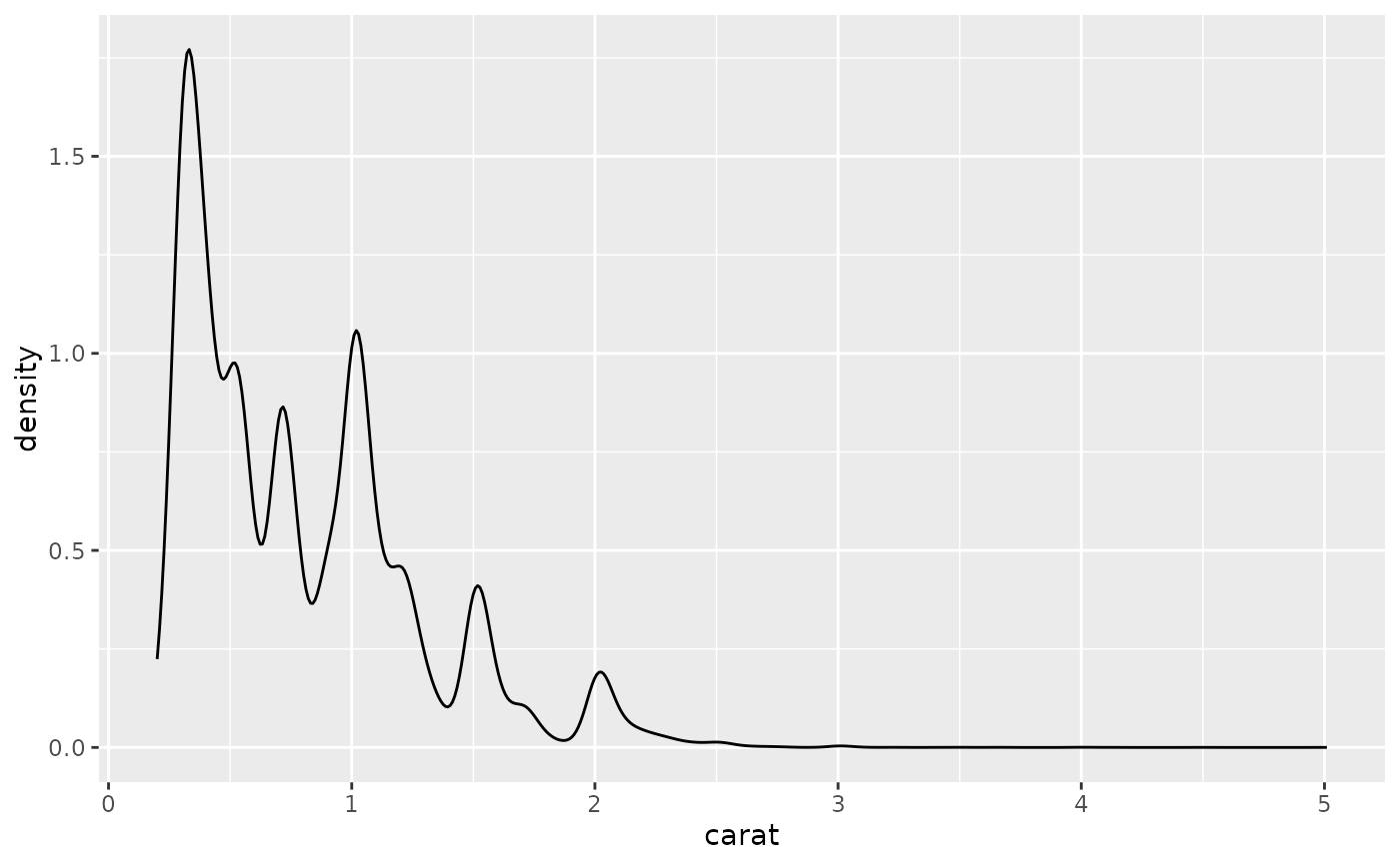
ggplot(diamonds, aes(carat)) +
geom_density()
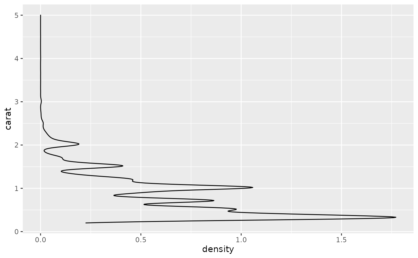
 # Map the values to y to flip the orientation
ggplot(diamonds, aes(y = carat)) +
geom_density()
# Map the values to y to flip the orientation
ggplot(diamonds, aes(y = carat)) +
geom_density()
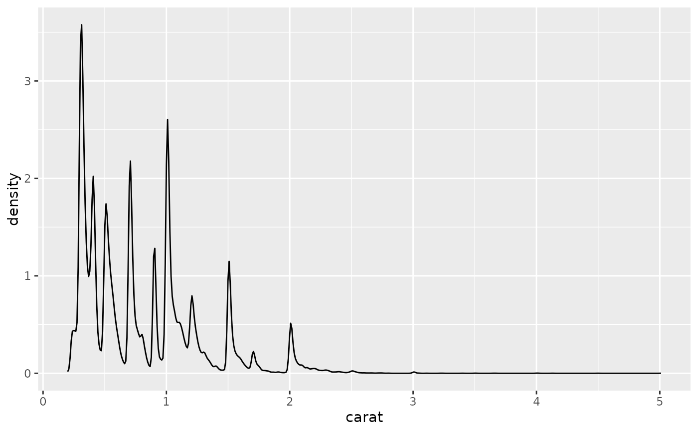
 ggplot(diamonds, aes(carat)) +
geom_density(adjust = 1/5)
ggplot(diamonds, aes(carat)) +
geom_density(adjust = 1/5)
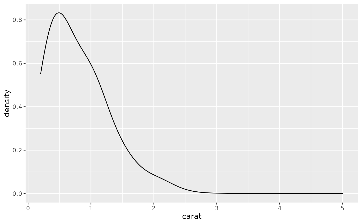
 ggplot(diamonds, aes(carat)) +
geom_density(adjust = 5)
ggplot(diamonds, aes(carat)) +
geom_density(adjust = 5)
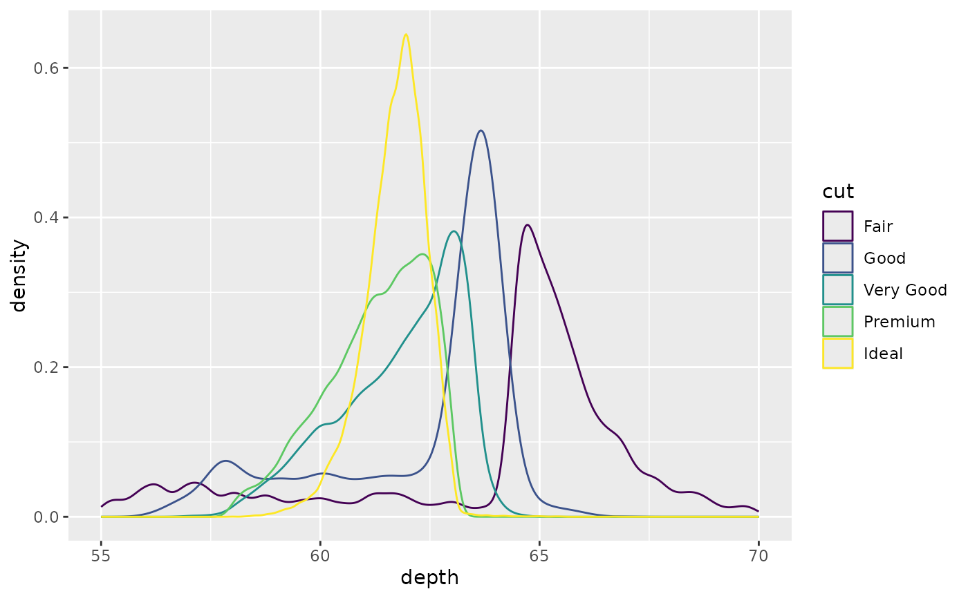
 ggplot(diamonds, aes(depth, colour = cut)) +
geom_density() +
xlim(55, 70)
#> Warning: Removed 45 rows containing non-finite outside the scale range
#> (`stat_density()`).
ggplot(diamonds, aes(depth, colour = cut)) +
geom_density() +
xlim(55, 70)
#> Warning: Removed 45 rows containing non-finite outside the scale range
#> (`stat_density()`).
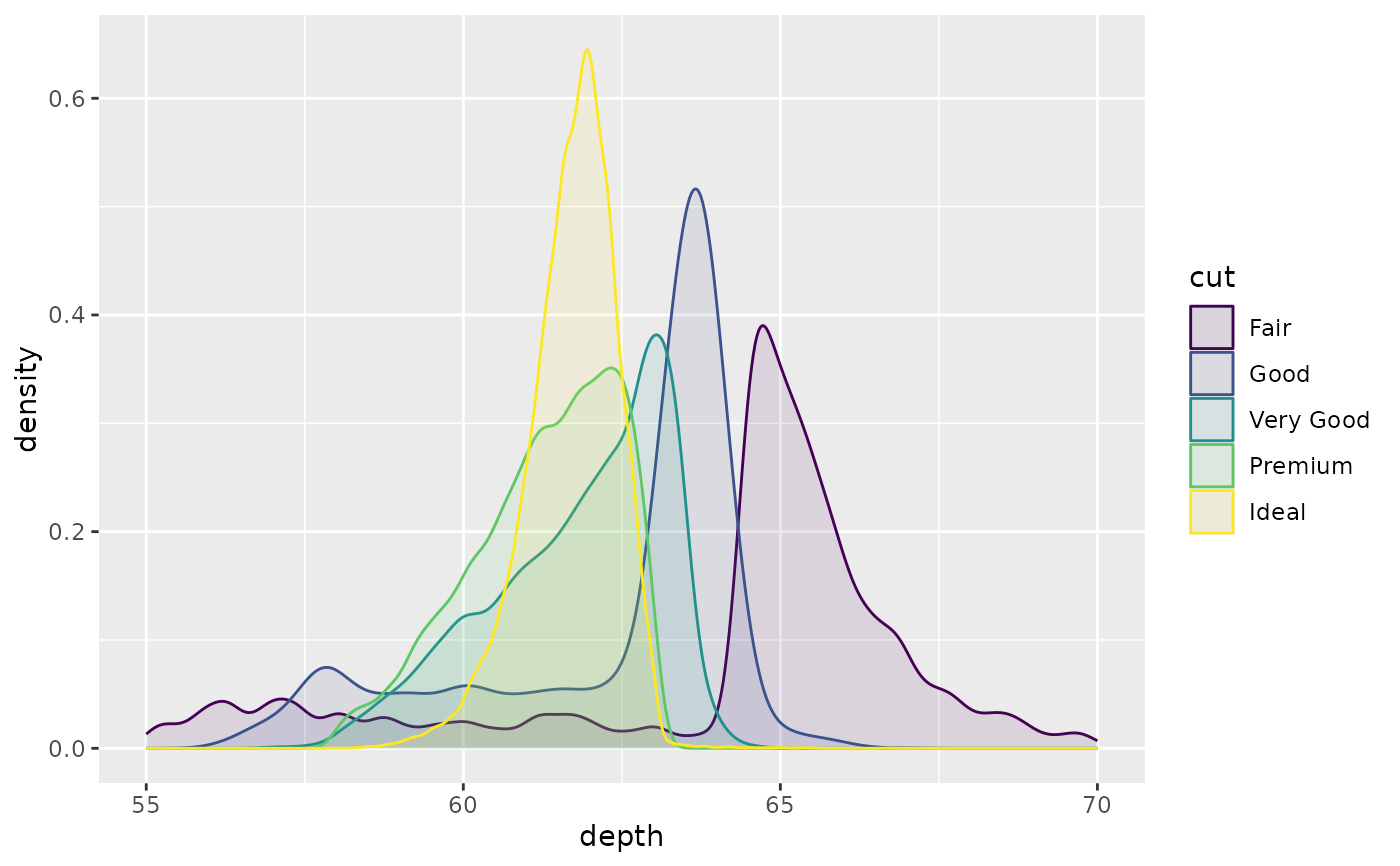
 ggplot(diamonds, aes(depth, fill = cut, colour = cut)) +
geom_density(alpha = 0.1) +
xlim(55, 70)
#> Warning: Removed 45 rows containing non-finite outside the scale range
#> (`stat_density()`).
ggplot(diamonds, aes(depth, fill = cut, colour = cut)) +
geom_density(alpha = 0.1) +
xlim(55, 70)
#> Warning: Removed 45 rows containing non-finite outside the scale range
#> (`stat_density()`).
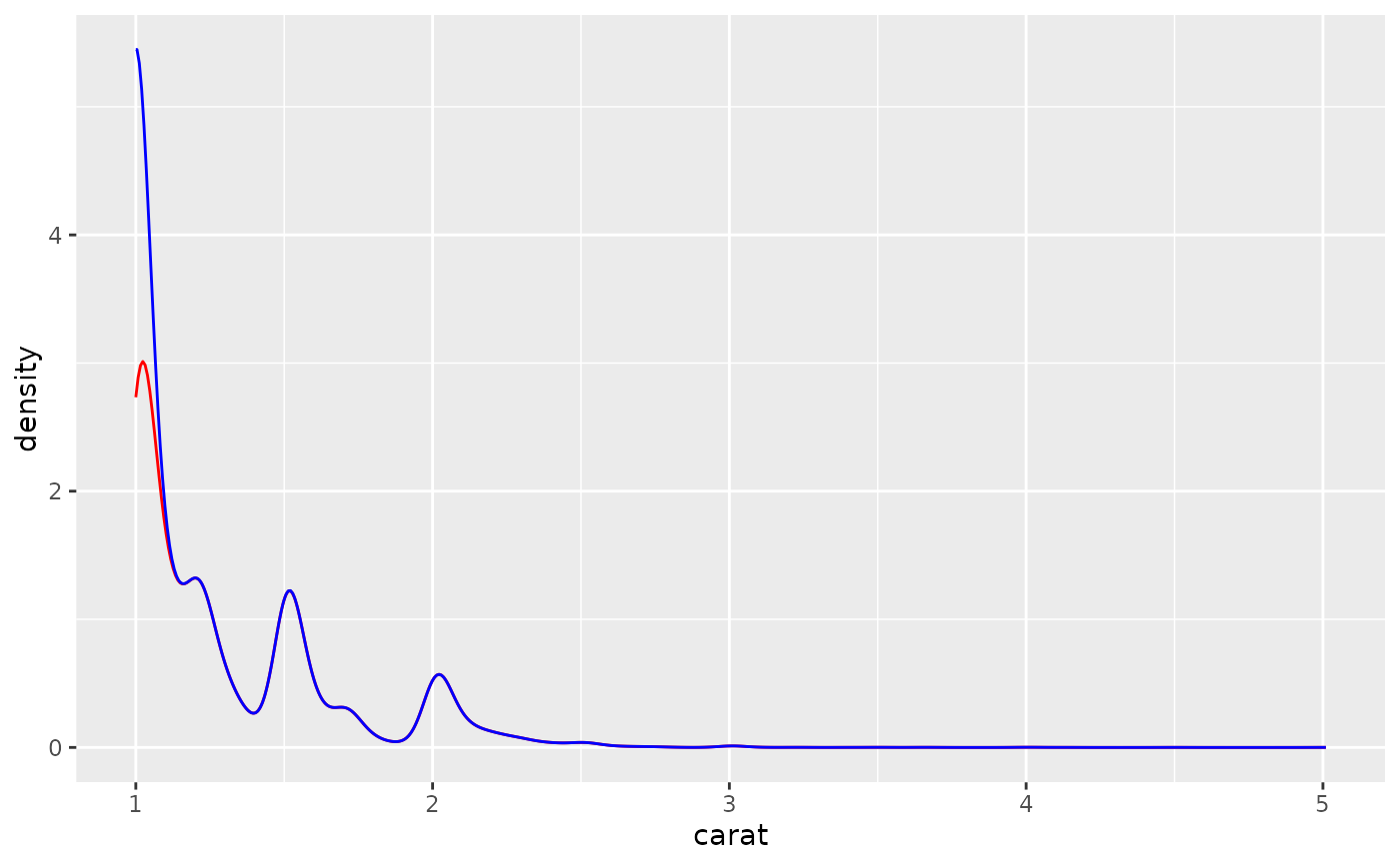
 # Use `bounds` to adjust computation for known data limits
big_diamonds <- diamonds[diamonds$carat >= 1, ]
ggplot(big_diamonds, aes(carat)) +
geom_density(color = 'red') +
geom_density(bounds = c(1, Inf), color = 'blue')
# Use `bounds` to adjust computation for known data limits
big_diamonds <- diamonds[diamonds$carat >= 1, ]
ggplot(big_diamonds, aes(carat)) +
geom_density(color = 'red') +
geom_density(bounds = c(1, Inf), color = 'blue')
 # \donttest{
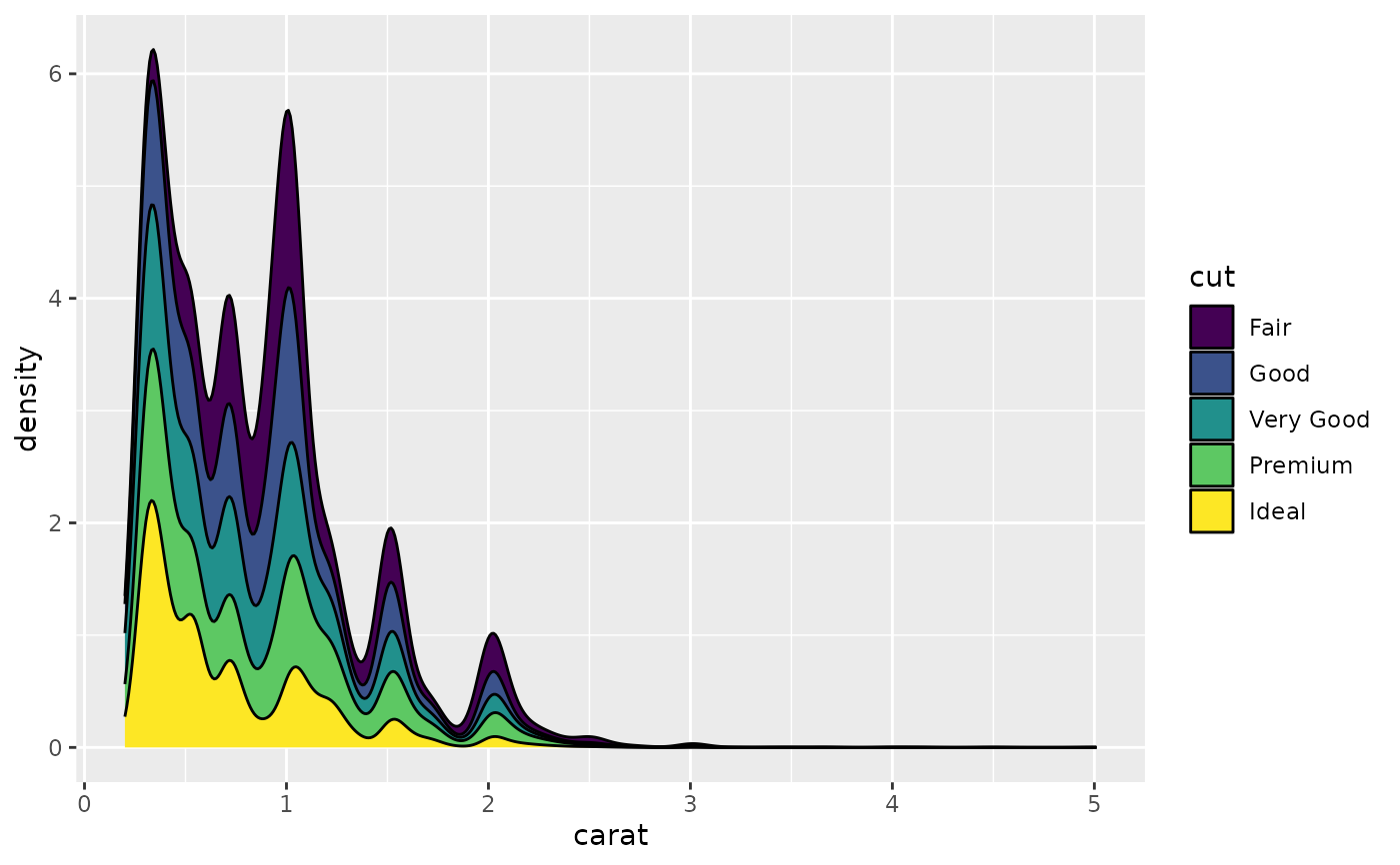
# Stacked density plots: if you want to create a stacked density plot, you
# probably want to 'count' (density * n) variable instead of the default
# density
# Loses marginal densities
ggplot(diamonds, aes(carat, fill = cut)) +
geom_density(position = "stack")
# \donttest{
# Stacked density plots: if you want to create a stacked density plot, you
# probably want to 'count' (density * n) variable instead of the default
# density
# Loses marginal densities
ggplot(diamonds, aes(carat, fill = cut)) +
geom_density(position = "stack")
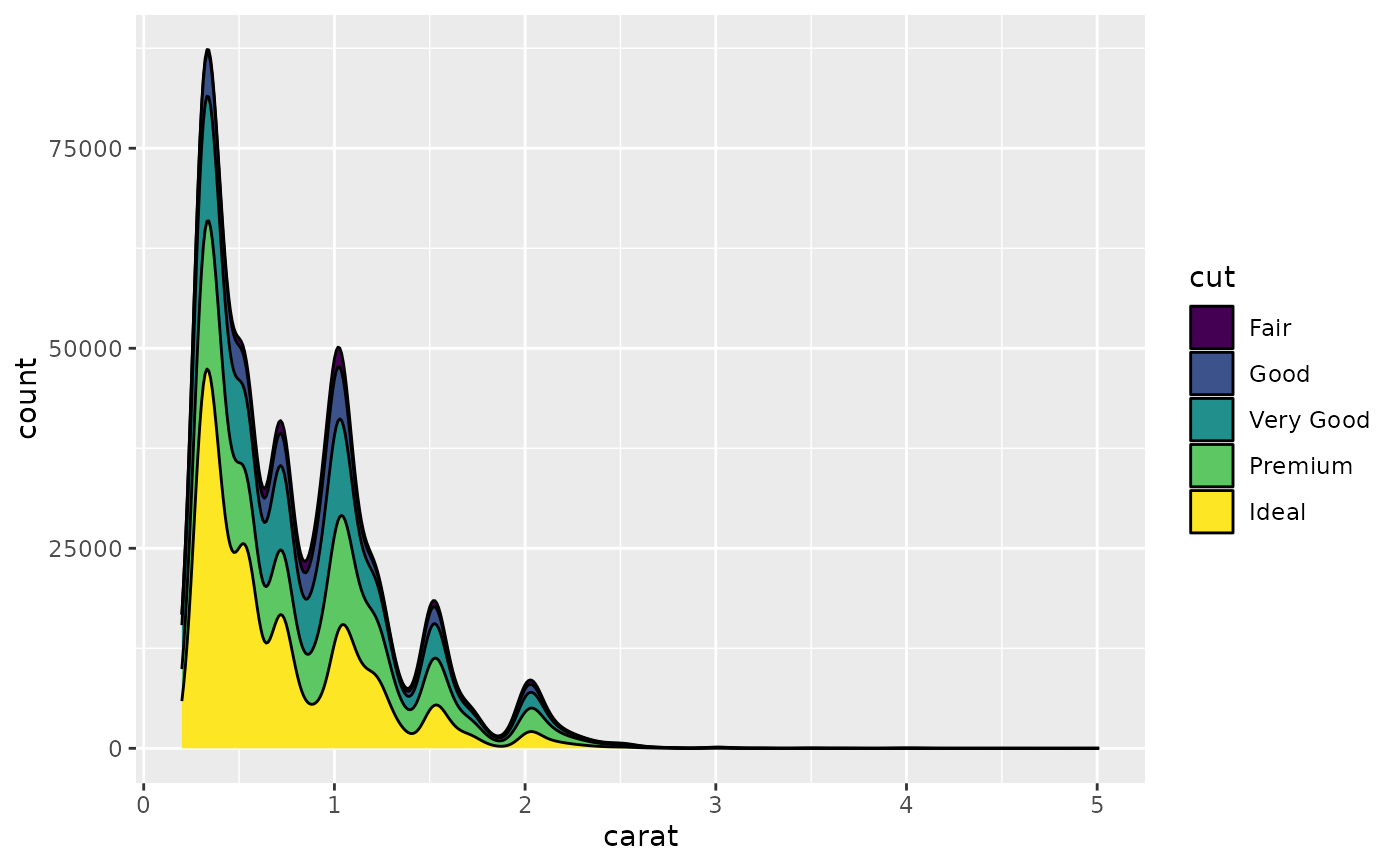
 # Preserves marginal densities
ggplot(diamonds, aes(carat, after_stat(count), fill = cut)) +
geom_density(position = "stack")
# Preserves marginal densities
ggplot(diamonds, aes(carat, after_stat(count), fill = cut)) +
geom_density(position = "stack")
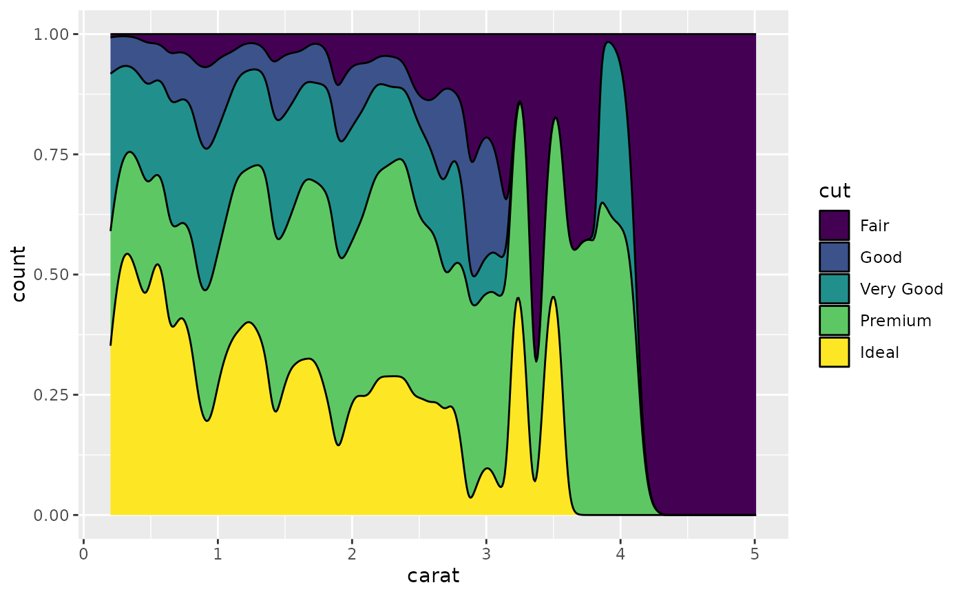
 # You can use position="fill" to produce a conditional density estimate
ggplot(diamonds, aes(carat, after_stat(count), fill = cut)) +
geom_density(position = "fill")
# You can use position="fill" to produce a conditional density estimate
ggplot(diamonds, aes(carat, after_stat(count), fill = cut)) +
geom_density(position = "fill")
 # }
# }