A box and whiskers plot (in the style of Tukey)
Source:R/geom-boxplot.R, R/stat-boxplot.R
geom_boxplot.RdThe boxplot compactly displays the distribution of a continuous variable. It visualises five summary statistics (the median, two hinges and two whiskers), and all "outlying" points individually.
Usage
geom_boxplot(
  mapping = NULL,
  data = NULL,
  stat = "boxplot",
  position = "dodge2",
  ...,
  outliers = TRUE,
  outlier.colour = NULL,
  outlier.color = NULL,
  outlier.fill = NULL,
  outlier.shape = NULL,
  outlier.size = NULL,
  outlier.stroke = 0.5,
  outlier.alpha = NULL,
  whisker.colour = NULL,
  whisker.color = NULL,
  whisker.linetype = NULL,
  whisker.linewidth = NULL,
  staple.colour = NULL,
  staple.color = NULL,
  staple.linetype = NULL,
  staple.linewidth = NULL,
  median.colour = NULL,
  median.color = NULL,
  median.linetype = NULL,
  median.linewidth = NULL,
  box.colour = NULL,
  box.color = NULL,
  box.linetype = NULL,
  box.linewidth = NULL,
  notch = FALSE,
  notchwidth = 0.5,
  staplewidth = 0,
  varwidth = FALSE,
  na.rm = FALSE,
  orientation = NA,
  show.legend = NA,
  inherit.aes = TRUE
)

stat_boxplot(
  mapping = NULL,
  data = NULL,
  geom = "boxplot",
  position = "dodge2",
  ...,
  orientation = NA,
  coef = 1.5,
  quantile.type = 7,
  na.rm = FALSE,
  show.legend = NA,
  inherit.aes = TRUE
)
Arguments
- mapping
Set of aesthetic mappings created by
aes(). If specified andinherit.aes = TRUE(the default), it is combined with the default mapping at the top level of the plot. You must supplymappingif there is no plot mapping.- data
The data to be displayed in this layer. There are three options:
If
NULL, the default, the data is inherited from the plot data as specified in the call toggplot().A
data.frame, or other object, will override the plot data. All objects will be fortified to produce a data frame. Seefortify()for which variables will be created.A
functionwill be called with a single argument, the plot data. The return value must be adata.frame, and will be used as the layer data. Afunctioncan be created from aformula(e.g.~ head(.x, 10)).- position
A position adjustment to use on the data for this layer. This can be used in various ways, including to prevent overplotting and improving the display. The
positionargument accepts the following:The result of calling a position function, such as
position_jitter(). This method allows for passing extra arguments to the position.A string naming the position adjustment. To give the position as a string, strip the function name of the
position_prefix. For example, to useposition_jitter(), give the position as"jitter".For more information and other ways to specify the position, see the layer position documentation.
- ...
Other arguments passed on to
layer()'sparamsargument. These arguments broadly fall into one of 4 categories below. Notably, further arguments to thepositionargument, or aesthetics that are required can not be passed through.... Unknown arguments that are not part of the 4 categories below are ignored.Static aesthetics that are not mapped to a scale, but are at a fixed value and apply to the layer as a whole. For example,
colour = "red"orlinewidth = 3. The geom's documentation has an Aesthetics section that lists the available options. The 'required' aesthetics cannot be passed on to theparams. Please note that while passing unmapped aesthetics as vectors is technically possible, the order and required length is not guaranteed to be parallel to the input data.When constructing a layer using a
stat_*()function, the...argument can be used to pass on parameters to thegeompart of the layer. An example of this isstat_density(geom = "area", outline.type = "both"). The geom's documentation lists which parameters it can accept.Inversely, when constructing a layer using a
geom_*()function, the...argument can be used to pass on parameters to thestatpart of the layer. An example of this isgeom_area(stat = "density", adjust = 0.5). The stat's documentation lists which parameters it can accept.The
key_glyphargument oflayer()may also be passed on through.... This can be one of the functions described as key glyphs, to change the display of the layer in the legend.
- outliers
Whether to display (
TRUE) or discard (FALSE) outliers from the plot. Hiding or discarding outliers can be useful when, for example, raw data points need to be displayed on top of the boxplot. By discarding outliers, the axis limits will adapt to the box and whiskers only, not the full data range. If outliers need to be hidden and the axes needs to show the full data range, please useoutlier.shape = NAinstead.- outlier.colour, outlier.color, outlier.fill, outlier.shape, outlier.size, outlier.stroke, outlier.alpha
Default aesthetics for outliers. Set to
NULLto inherit from the data's aesthetics.- whisker.colour, whisker.color, whisker.linetype, whisker.linewidth
Default aesthetics for the whiskers. Set to
NULLto inherit from the data's aesthetics.- staple.colour, staple.color, staple.linetype, staple.linewidth
Default aesthetics for the staples. Set to
NULLto inherit from the data's aesthetics. Note that staples don't appear unless thestaplewidthargument is set to a non-zero size.- median.colour, median.color, median.linetype, median.linewidth
Default aesthetics for the median line. Set to
NULLto inherit from the data's aesthetics.- box.colour, box.color, box.linetype, box.linewidth
Default aesthetics for the boxes. Set to
NULLto inherit from the data's aesthetics.- notch
If
FALSE(default) make a standard box plot. IfTRUE, make a notched box plot. Notches are used to compare groups; if the notches of two boxes do not overlap, this suggests that the medians are significantly different.- notchwidth
For a notched box plot, width of the notch relative to the body (defaults to
notchwidth = 0.5).- staplewidth
The relative width of staples to the width of the box. Staples mark the ends of the whiskers with a line.
- varwidth
If
FALSE(default) make a standard box plot. IfTRUE, boxes are drawn with widths proportional to the square-roots of the number of observations in the groups (possibly weighted, using theweightaesthetic).- na.rm
If
FALSE, the default, missing values are removed with a warning. IfTRUE, missing values are silently removed.- orientation
The orientation of the layer. The default (
NA) automatically determines the orientation from the aesthetic mapping. In the rare event that this fails it can be given explicitly by settingorientationto either"x"or"y". See the Orientation section for more detail.- show.legend
logical. Should this layer be included in the legends?
NA, the default, includes if any aesthetics are mapped.FALSEnever includes, andTRUEalways includes. It can also be a named logical vector to finely select the aesthetics to display. To include legend keys for all levels, even when no data exists, useTRUE. IfNA, all levels are shown in legend, but unobserved levels are omitted.- inherit.aes
If
FALSE, overrides the default aesthetics, rather than combining with them. This is most useful for helper functions that define both data and aesthetics and shouldn't inherit behaviour from the default plot specification, e.g.annotation_borders().- geom, stat
Use to override the default connection between
geom_boxplot()andstat_boxplot(). For more information about overriding these connections, see how the stat and geom arguments work.- coef
Length of the whiskers as multiple of IQR. Defaults to 1.5.
- quantile.type
An integer between 1 and 9 setting the quantile algorithm per
stats::quantile(type). Defaults to7
Note
In the unlikely event you specify both US and UK spellings of colour, the US spelling will take precedence.
Orientation
This geom treats each axis differently and, thus, can thus have two orientations. Often the orientation is easy to deduce from a combination of the given mappings and the types of positional scales in use. Thus, ggplot2 will by default try to guess which orientation the layer should have. Under rare circumstances, the orientation is ambiguous and guessing may fail. In that case the orientation can be specified directly using the orientation parameter, which can be either "x" or "y". The value gives the axis that the geom should run along, "x" being the default orientation you would expect for the geom.
Summary statistics
The lower and upper hinges correspond to the first and third quartiles
(the 25th and 75th percentiles). This differs slightly from the method used
by the boxplot() function, and may be apparent with small samples.
See boxplot.stats() for more information on how hinge
positions are calculated for boxplot().
The upper whisker extends from the hinge to the largest value no further than 1.5 * IQR from the hinge (where IQR is the inter-quartile range, or distance between the first and third quartiles). The lower whisker extends from the hinge to the smallest value at most 1.5 * IQR of the hinge. Data beyond the end of the whiskers are called "outlying" points and are plotted individually.
In a notched box plot, the notches extend 1.58 * IQR / sqrt(n).
This gives a roughly 95% confidence interval for comparing medians.
See McGill et al. (1978) for more details.
Computed variables
These are calculated by the 'stat' part of layers and can be accessed with delayed evaluation. stat_boxplot() provides the following variables, some of which depend on the orientation:
after_stat(width)
width of boxplot.after_stat(ymin)orafter_stat(xmin)
lower whisker = smallest observation greater than or equal to lower hinger - 1.5 * IQR.after_stat(lower)orafter_stat(xlower)
lower hinge, 25% quantile.after_stat(notchlower)
lower edge of notch = median - 1.58 * IQR / sqrt(n).after_stat(middle)orafter_stat(xmiddle)
median, 50% quantile.after_stat(notchupper)
upper edge of notch = median + 1.58 * IQR / sqrt(n).after_stat(upper)orafter_stat(xupper)
upper hinge, 75% quantile.after_stat(ymax)orafter_stat(xmax)
upper whisker = largest observation less than or equal to upper hinger + 1.5 * IQR.
References
McGill, R., Tukey, J. W. and Larsen, W. A. (1978) Variations of box plots. The American Statistician 32, 12-16.
See also
geom_quantile() for continuous x,
geom_violin() for a richer display of the distribution, and
geom_jitter() for a useful technique for small data.
Aesthetics
geom_boxplot() understands the following aesthetics. Required aesthetics are displayed in bold and defaults are displayed for optional aesthetics:
| • | x or y | |
| • | lower or xlower | |
| • | upper or xupper | |
| • | middle or xmiddle | |
| • | ymin or xmin | |
| • | ymax or xmax | |
| • | alpha | → NA |
| • | colour | → via theme() |
| • | fill | → via theme() |
| • | group | → inferred |
| • | linetype | → via theme() |
| • | linewidth | → via theme() |
| • | shape | → via theme() |
| • | size | → via theme() |
| • | weight | → 1 |
| • | width | → 0.9 |
Learn more about setting these aesthetics in vignette("ggplot2-specs").
Examples
p <- ggplot(mpg, aes(class, hwy))
p + geom_boxplot()
 # Orientation follows the discrete axis
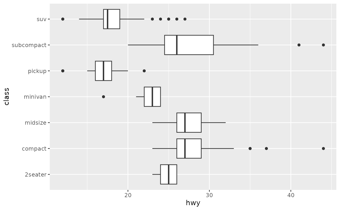
ggplot(mpg, aes(hwy, class)) + geom_boxplot()
# Orientation follows the discrete axis
ggplot(mpg, aes(hwy, class)) + geom_boxplot()
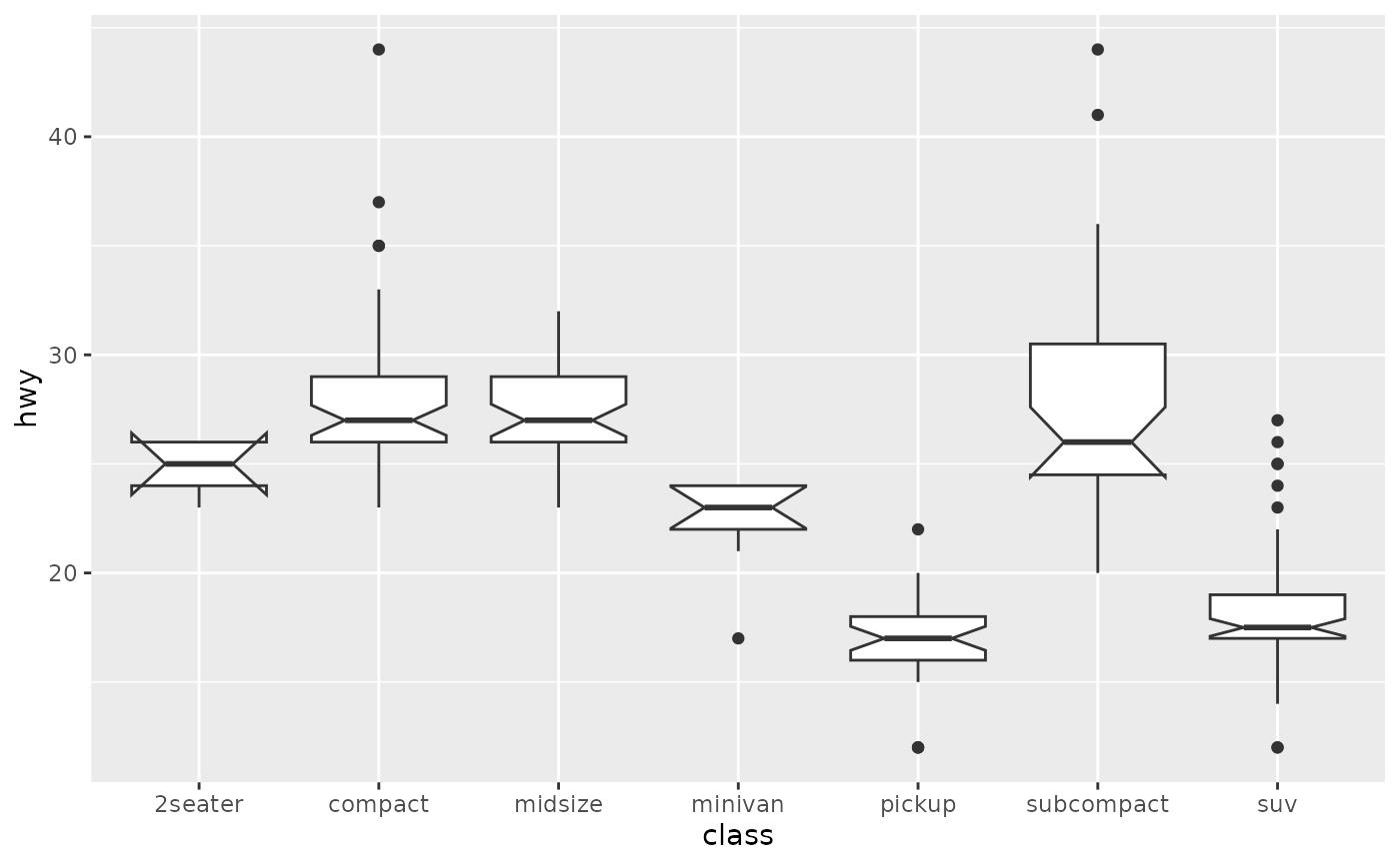
 p + geom_boxplot(notch = TRUE)
#> Notch went outside hinges
#> ℹ Do you want `notch = FALSE`?
#> Notch went outside hinges
#> ℹ Do you want `notch = FALSE`?
p + geom_boxplot(notch = TRUE)
#> Notch went outside hinges
#> ℹ Do you want `notch = FALSE`?
#> Notch went outside hinges
#> ℹ Do you want `notch = FALSE`?
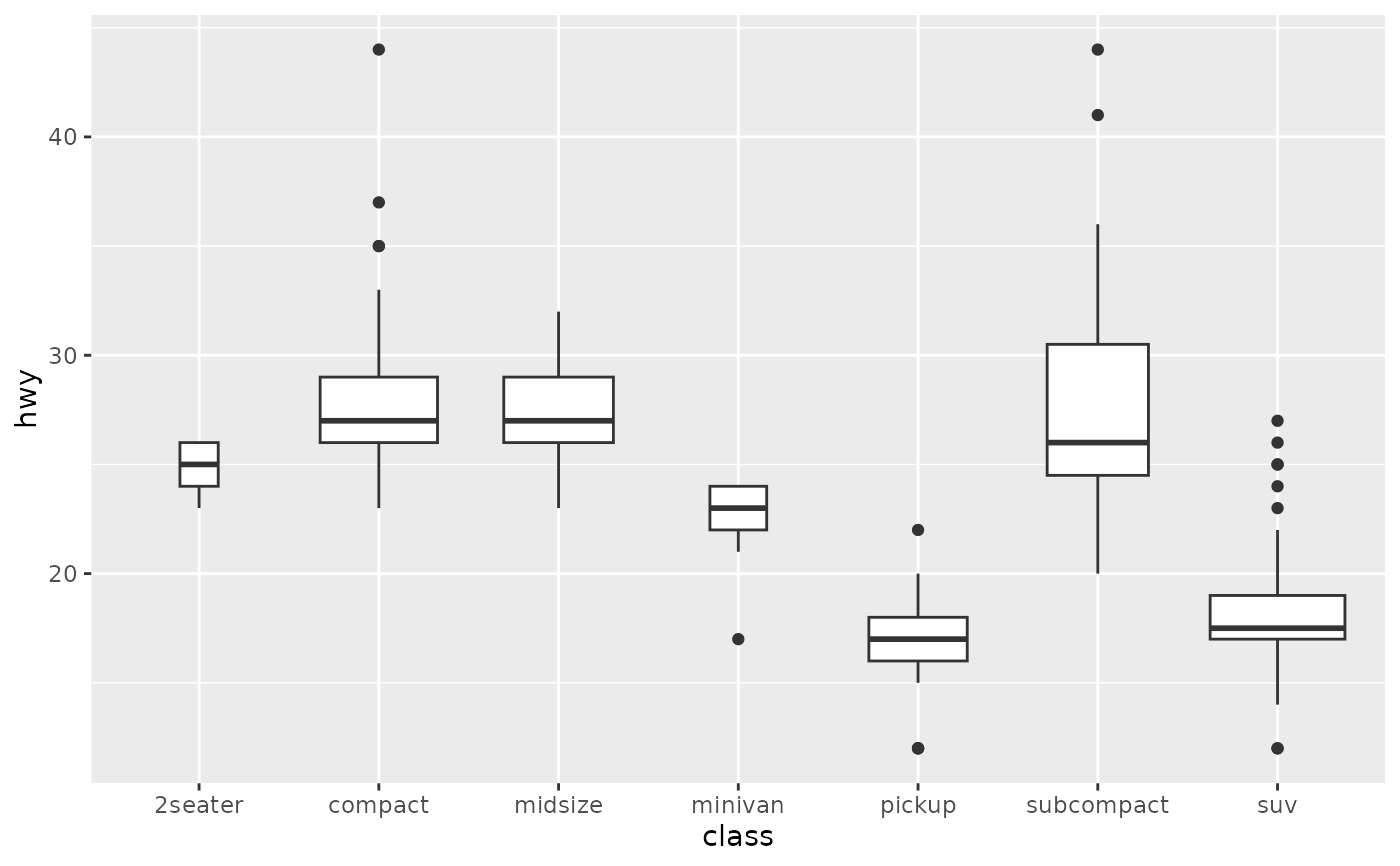
 p + geom_boxplot(varwidth = TRUE)
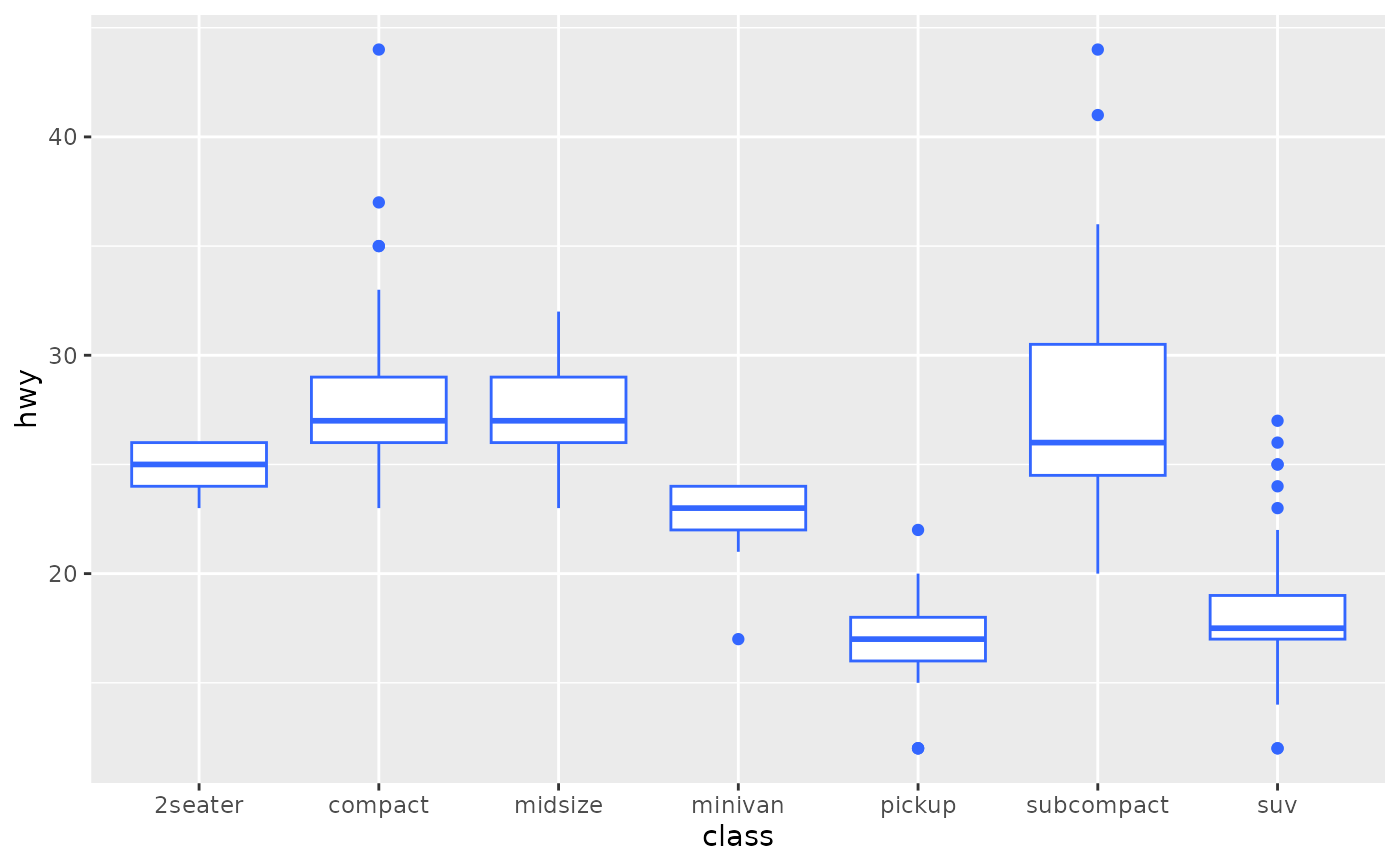
 p + geom_boxplot(fill = "white", colour = "#3366FF")
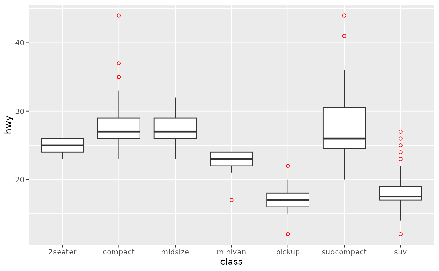
 # By default, outlier points match the colour of the box. Use
# outlier.colour to override
p + geom_boxplot(outlier.colour = "red", outlier.shape = 1)
# By default, outlier points match the colour of the box. Use
# outlier.colour to override
p + geom_boxplot(outlier.colour = "red", outlier.shape = 1)
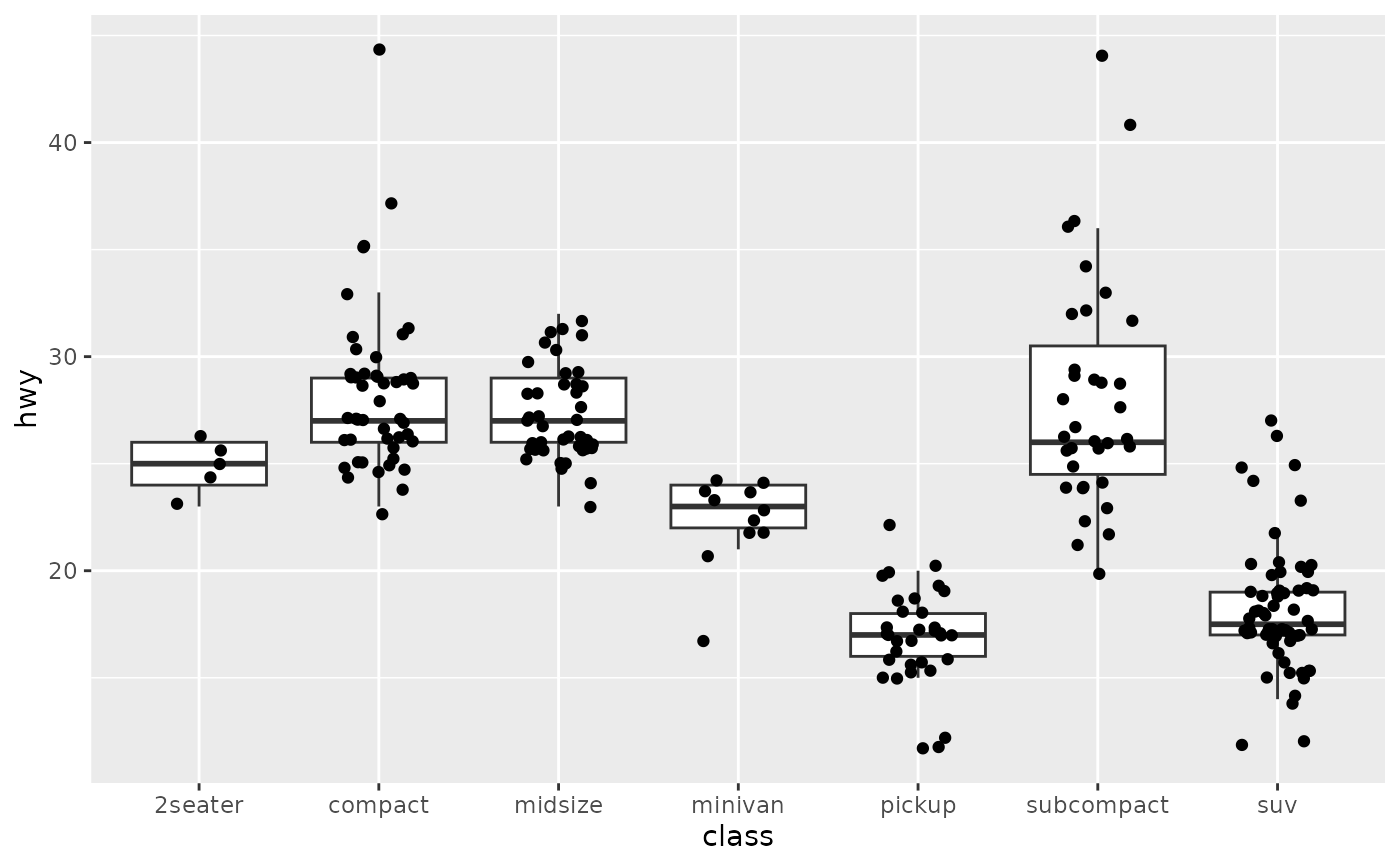
 # Remove outliers when overlaying boxplot with original data points
p + geom_boxplot(outlier.shape = NA) + geom_jitter(width = 0.2)
# Remove outliers when overlaying boxplot with original data points
p + geom_boxplot(outlier.shape = NA) + geom_jitter(width = 0.2)
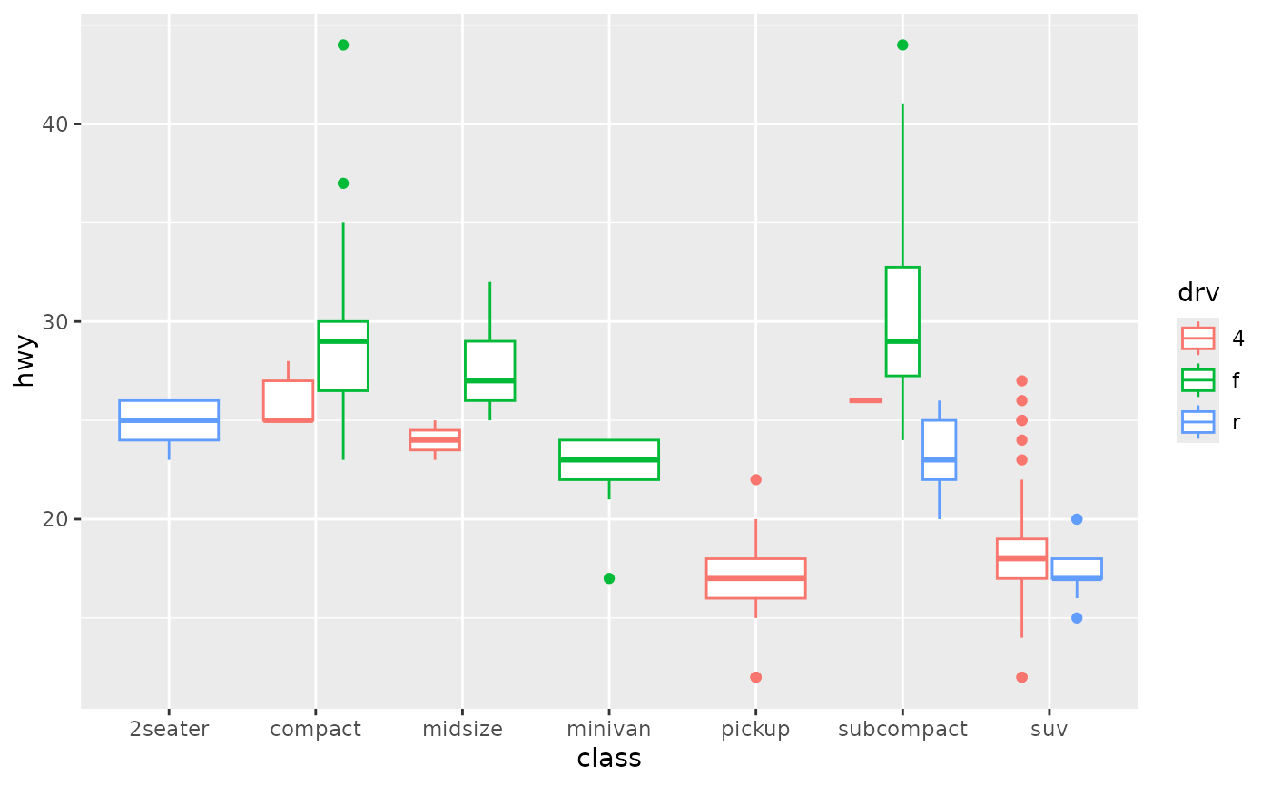
 # Boxplots are automatically dodged when any aesthetic is a factor
p + geom_boxplot(aes(colour = drv))
# Boxplots are automatically dodged when any aesthetic is a factor
p + geom_boxplot(aes(colour = drv))
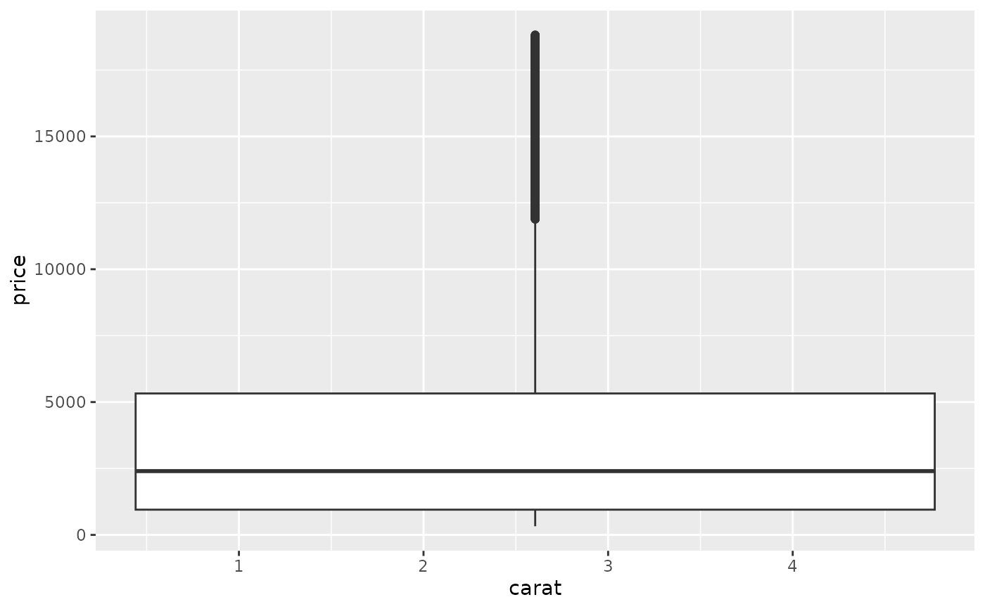
 # You can also use boxplots with continuous x, as long as you supply
# a grouping variable. cut_width is particularly useful
ggplot(diamonds, aes(carat, price)) +
geom_boxplot()
#> Warning: Orientation is not uniquely specified when both the x and y aesthetics
#> are continuous. Picking default orientation 'x'.
#> Warning: Continuous x aesthetic
#> ℹ did you forget `aes(group = ...)`?
# You can also use boxplots with continuous x, as long as you supply
# a grouping variable. cut_width is particularly useful
ggplot(diamonds, aes(carat, price)) +
geom_boxplot()
#> Warning: Orientation is not uniquely specified when both the x and y aesthetics
#> are continuous. Picking default orientation 'x'.
#> Warning: Continuous x aesthetic
#> ℹ did you forget `aes(group = ...)`?
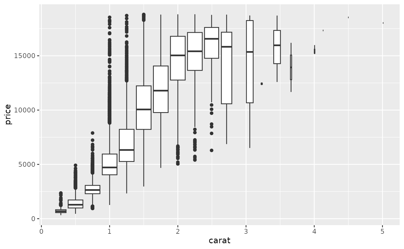
 ggplot(diamonds, aes(carat, price)) +
geom_boxplot(aes(group = cut_width(carat, 0.25)))
#> Warning: Orientation is not uniquely specified when both the x and y aesthetics
#> are continuous. Picking default orientation 'x'.
ggplot(diamonds, aes(carat, price)) +
geom_boxplot(aes(group = cut_width(carat, 0.25)))
#> Warning: Orientation is not uniquely specified when both the x and y aesthetics
#> are continuous. Picking default orientation 'x'.
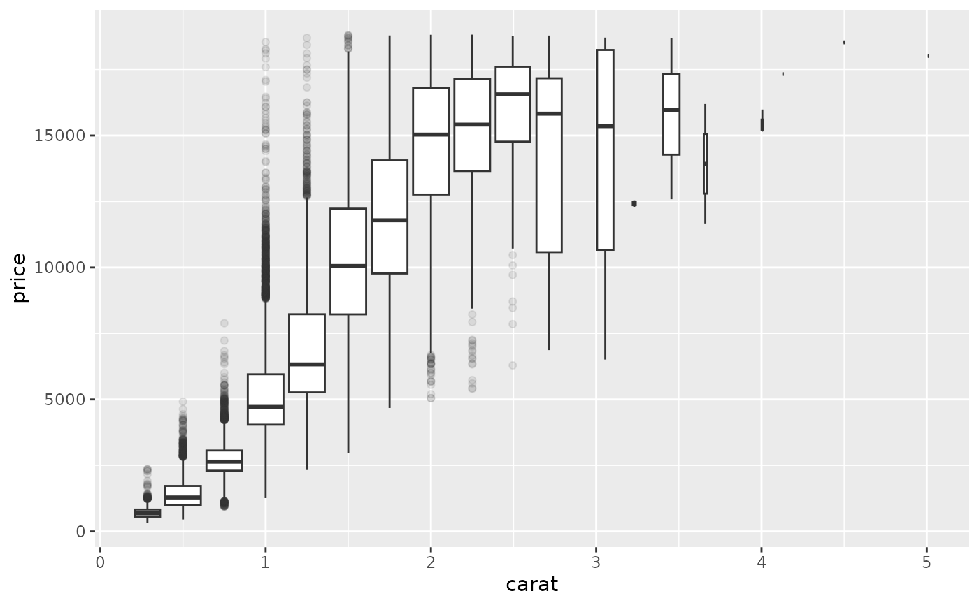
 # Adjust the transparency of outliers using outlier.alpha
ggplot(diamonds, aes(carat, price)) +
geom_boxplot(aes(group = cut_width(carat, 0.25)), outlier.alpha = 0.1)
#> Warning: Orientation is not uniquely specified when both the x and y aesthetics
#> are continuous. Picking default orientation 'x'.
# Adjust the transparency of outliers using outlier.alpha
ggplot(diamonds, aes(carat, price)) +
geom_boxplot(aes(group = cut_width(carat, 0.25)), outlier.alpha = 0.1)
#> Warning: Orientation is not uniquely specified when both the x and y aesthetics
#> are continuous. Picking default orientation 'x'.
 # \donttest{
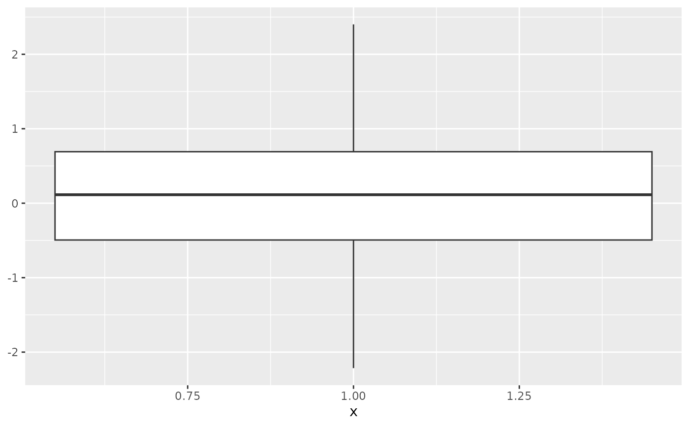
# It's possible to draw a boxplot with your own computations if you
# use stat = "identity":
set.seed(1)
y <- rnorm(100)
df <- data.frame(
x = 1,
y0 = min(y),
y25 = quantile(y, 0.25),
y50 = median(y),
y75 = quantile(y, 0.75),
y100 = max(y)
)
ggplot(df, aes(x)) +
geom_boxplot(
aes(ymin = y0, lower = y25, middle = y50, upper = y75, ymax = y100),
stat = "identity"
)
# \donttest{
# It's possible to draw a boxplot with your own computations if you
# use stat = "identity":
set.seed(1)
y <- rnorm(100)
df <- data.frame(
x = 1,
y0 = min(y),
y25 = quantile(y, 0.25),
y50 = median(y),
y75 = quantile(y, 0.75),
y100 = max(y)
)
ggplot(df, aes(x)) +
geom_boxplot(
aes(ymin = y0, lower = y25, middle = y50, upper = y75, ymax = y100),
stat = "identity"
)
 # }
# }