geom_path() connects the observations in the order in which they appear
in the data. geom_line() connects them in order of the variable on the
x axis. geom_step() creates a stairstep plot, highlighting exactly
when changes occur. The group aesthetic determines which cases are
connected together.
Usage
geom_path(
  mapping = NULL,
  data = NULL,
  stat = "identity",
  position = "identity",
  ...,
  arrow = NULL,
  arrow.fill = NULL,
  lineend = "butt",
  linejoin = "round",
  linemitre = 10,
  na.rm = FALSE,
  show.legend = NA,
  inherit.aes = TRUE
)

geom_line(
  mapping = NULL,
  data = NULL,
  stat = "identity",
  position = "identity",
  ...,
  orientation = NA,
  arrow = NULL,
  arrow.fill = NULL,
  lineend = "butt",
  linejoin = "round",
  linemitre = 10,
  na.rm = FALSE,
  show.legend = NA,
  inherit.aes = TRUE
)

geom_step(
  mapping = NULL,
  data = NULL,
  stat = "identity",
  position = "identity",
  ...,
  orientation = NA,
  lineend = "butt",
  linejoin = "round",
  linemitre = 10,
  arrow = NULL,
  arrow.fill = NULL,
  direction = "hv",
  na.rm = FALSE,
  show.legend = NA,
  inherit.aes = TRUE
)
Arguments
- mapping
Set of aesthetic mappings created by
aes(). If specified andinherit.aes = TRUE(the default), it is combined with the default mapping at the top level of the plot. You must supplymappingif there is no plot mapping.- data
The data to be displayed in this layer. There are three options:
If
NULL, the default, the data is inherited from the plot data as specified in the call toggplot().A
data.frame, or other object, will override the plot data. All objects will be fortified to produce a data frame. Seefortify()for which variables will be created.A
functionwill be called with a single argument, the plot data. The return value must be adata.frame, and will be used as the layer data. Afunctioncan be created from aformula(e.g.~ head(.x, 10)).- stat
The statistical transformation to use on the data for this layer. When using a
geom_*()function to construct a layer, thestatargument can be used to override the default coupling between geoms and stats. Thestatargument accepts the following:A
Statggproto subclass, for exampleStatCount.A string naming the stat. To give the stat as a string, strip the function name of the
stat_prefix. For example, to usestat_count(), give the stat as"count".For more information and other ways to specify the stat, see the layer stat documentation.
- position
A position adjustment to use on the data for this layer. This can be used in various ways, including to prevent overplotting and improving the display. The
positionargument accepts the following:The result of calling a position function, such as
position_jitter(). This method allows for passing extra arguments to the position.A string naming the position adjustment. To give the position as a string, strip the function name of the
position_prefix. For example, to useposition_jitter(), give the position as"jitter".For more information and other ways to specify the position, see the layer position documentation.
- ...
Other arguments passed on to
layer()'sparamsargument. These arguments broadly fall into one of 4 categories below. Notably, further arguments to thepositionargument, or aesthetics that are required can not be passed through.... Unknown arguments that are not part of the 4 categories below are ignored.Static aesthetics that are not mapped to a scale, but are at a fixed value and apply to the layer as a whole. For example,
colour = "red"orlinewidth = 3. The geom's documentation has an Aesthetics section that lists the available options. The 'required' aesthetics cannot be passed on to theparams. Please note that while passing unmapped aesthetics as vectors is technically possible, the order and required length is not guaranteed to be parallel to the input data.When constructing a layer using a
stat_*()function, the...argument can be used to pass on parameters to thegeompart of the layer. An example of this isstat_density(geom = "area", outline.type = "both"). The geom's documentation lists which parameters it can accept.Inversely, when constructing a layer using a
geom_*()function, the...argument can be used to pass on parameters to thestatpart of the layer. An example of this isgeom_area(stat = "density", adjust = 0.5). The stat's documentation lists which parameters it can accept.The
key_glyphargument oflayer()may also be passed on through.... This can be one of the functions described as key glyphs, to change the display of the layer in the legend.
- arrow
Arrow specification, as created by
grid::arrow().- arrow.fill
fill colour to use for the arrow head (if closed).
NULLmeans usecolouraesthetic.- lineend
Line end style (round, butt, square).
- linejoin
Line join style (round, mitre, bevel).
- linemitre
Line mitre limit (number greater than 1).
- na.rm
If
FALSE, the default, missing values are removed with a warning. IfTRUE, missing values are silently removed.- show.legend
logical. Should this layer be included in the legends?
NA, the default, includes if any aesthetics are mapped.FALSEnever includes, andTRUEalways includes. It can also be a named logical vector to finely select the aesthetics to display. To include legend keys for all levels, even when no data exists, useTRUE. IfNA, all levels are shown in legend, but unobserved levels are omitted.- inherit.aes
If
FALSE, overrides the default aesthetics, rather than combining with them. This is most useful for helper functions that define both data and aesthetics and shouldn't inherit behaviour from the default plot specification, e.g.annotation_borders().- orientation
The orientation of the layer. The default (
NA) automatically determines the orientation from the aesthetic mapping. In the rare event that this fails it can be given explicitly by settingorientationto either"x"or"y". See the Orientation section for more detail.- direction
direction of stairs: 'vh' for vertical then horizontal, 'hv' for horizontal then vertical, or 'mid' for step half-way between adjacent x-values.
Details
An alternative parameterisation is geom_segment(), where each line
corresponds to a single case which provides the start and end coordinates.
Orientation
This geom treats each axis differently and, thus, can thus have two orientations. Often the orientation is easy to deduce from a combination of the given mappings and the types of positional scales in use. Thus, ggplot2 will by default try to guess which orientation the layer should have. Under rare circumstances, the orientation is ambiguous and guessing may fail. In that case the orientation can be specified directly using the orientation parameter, which can be either "x" or "y". The value gives the axis that the geom should run along, "x" being the default orientation you would expect for the geom.
Missing value handling
geom_path(), geom_line(), and geom_step() handle NA as follows:
If an
NAoccurs in the middle of a line, it breaks the line. No warning is shown, regardless of whetherna.rmisTRUEorFALSE.If an
NAoccurs at the start or the end of the line andna.rmisFALSE(default), theNAis removed with a warning.If an
NAoccurs at the start or the end of the line andna.rmisTRUE, theNAis removed silently, without warning.
See also
geom_polygon(): Filled paths (polygons);
geom_segment(): Line segments
Aesthetics
geom_path() understands the following aesthetics. Required aesthetics are displayed in bold and defaults are displayed for optional aesthetics:
| • | x | |
| • | y | |
| • | alpha | → NA |
| • | colour | → via theme() |
| • | group | → inferred |
| • | linetype | → via theme() |
| • | linewidth | → via theme() |
Learn more about setting these aesthetics in vignette("ggplot2-specs").
Examples
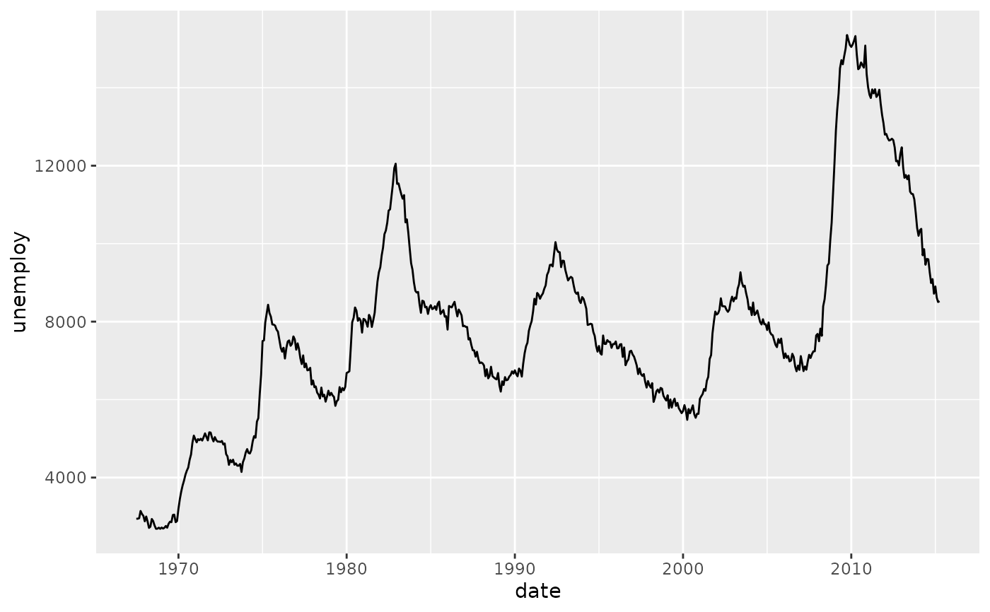
# geom_line() is suitable for time series
ggplot(economics, aes(date, unemploy)) + geom_line()
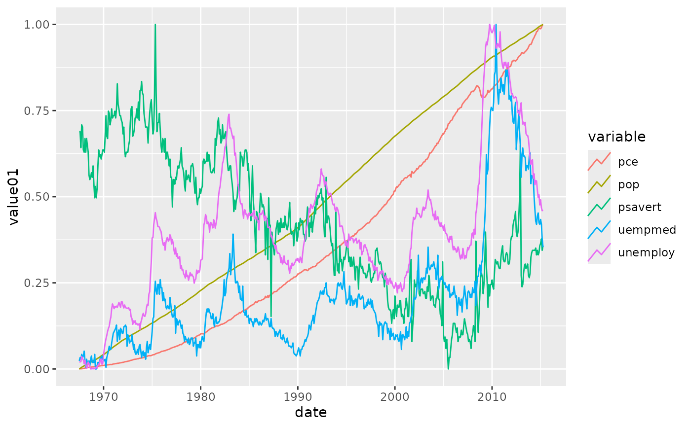
 # separate by colour and use "timeseries" legend key glyph
ggplot(economics_long, aes(date, value01, colour = variable)) +
geom_line(key_glyph = "timeseries")
# separate by colour and use "timeseries" legend key glyph
ggplot(economics_long, aes(date, value01, colour = variable)) +
geom_line(key_glyph = "timeseries")
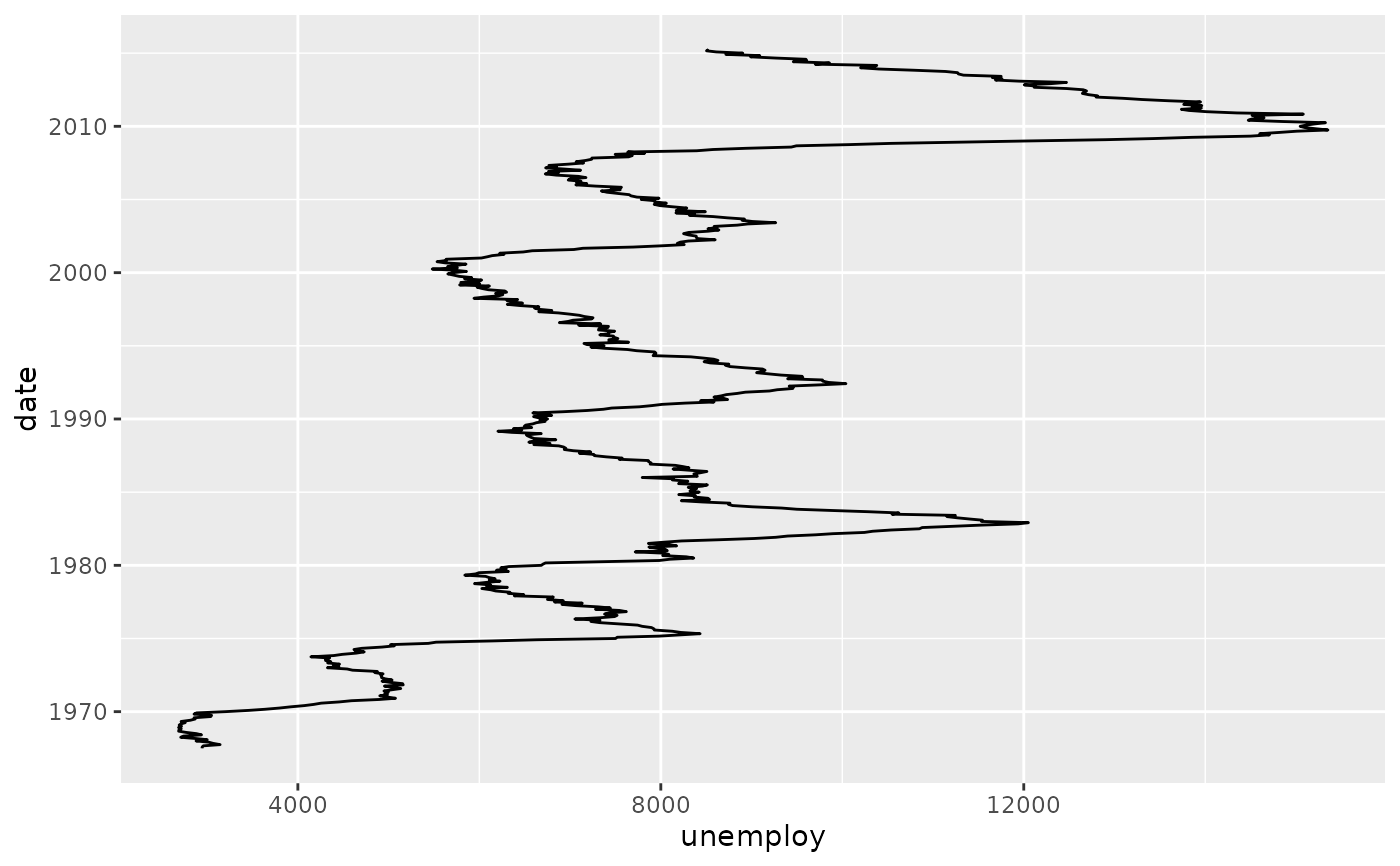
 # You can get a timeseries that run vertically by setting the orientation
ggplot(economics, aes(unemploy, date)) + geom_line(orientation = "y")
# You can get a timeseries that run vertically by setting the orientation
ggplot(economics, aes(unemploy, date)) + geom_line(orientation = "y")
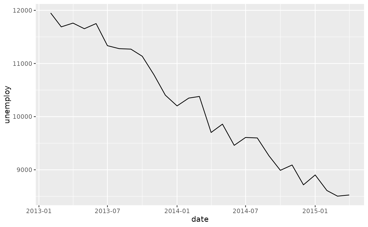
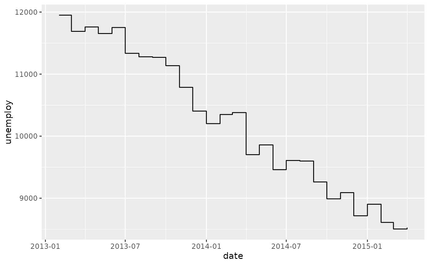
 # geom_step() is useful when you want to highlight exactly when
# the y value changes
recent <- economics[economics$date > as.Date("2013-01-01"), ]
ggplot(recent, aes(date, unemploy)) + geom_line()
# geom_step() is useful when you want to highlight exactly when
# the y value changes
recent <- economics[economics$date > as.Date("2013-01-01"), ]
ggplot(recent, aes(date, unemploy)) + geom_line()
 ggplot(recent, aes(date, unemploy)) + geom_step()
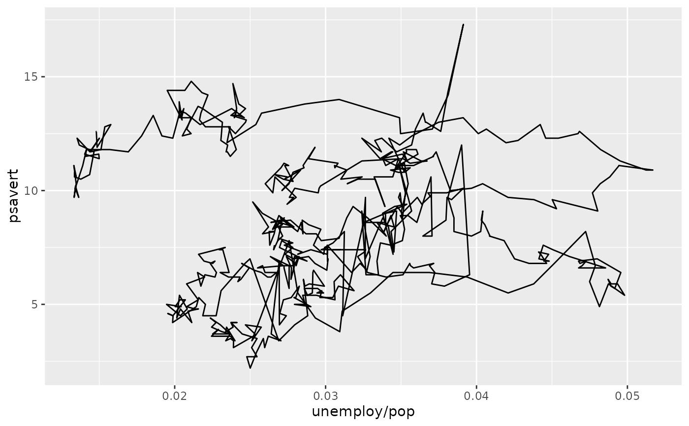
 # geom_path lets you explore how two variables are related over time,
# e.g. unemployment and personal savings rate
m <- ggplot(economics, aes(unemploy/pop, psavert))
m + geom_path()
# geom_path lets you explore how two variables are related over time,
# e.g. unemployment and personal savings rate
m <- ggplot(economics, aes(unemploy/pop, psavert))
m + geom_path()
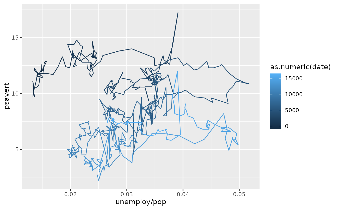
 m + geom_path(aes(colour = as.numeric(date)))
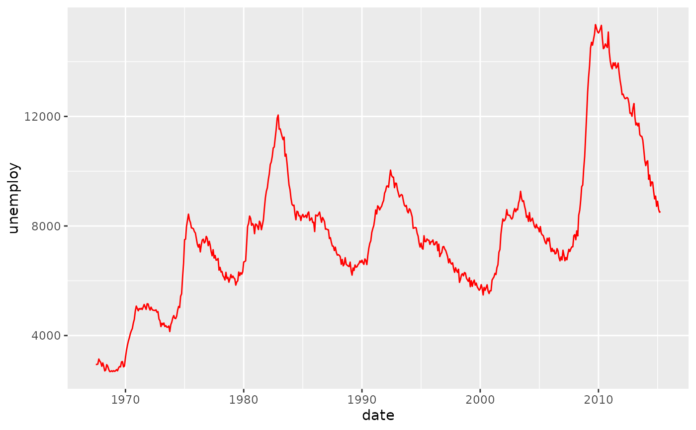
 # Changing parameters ----------------------------------------------
ggplot(economics, aes(date, unemploy)) +
geom_line(colour = "red")
# Changing parameters ----------------------------------------------
ggplot(economics, aes(date, unemploy)) +
geom_line(colour = "red")
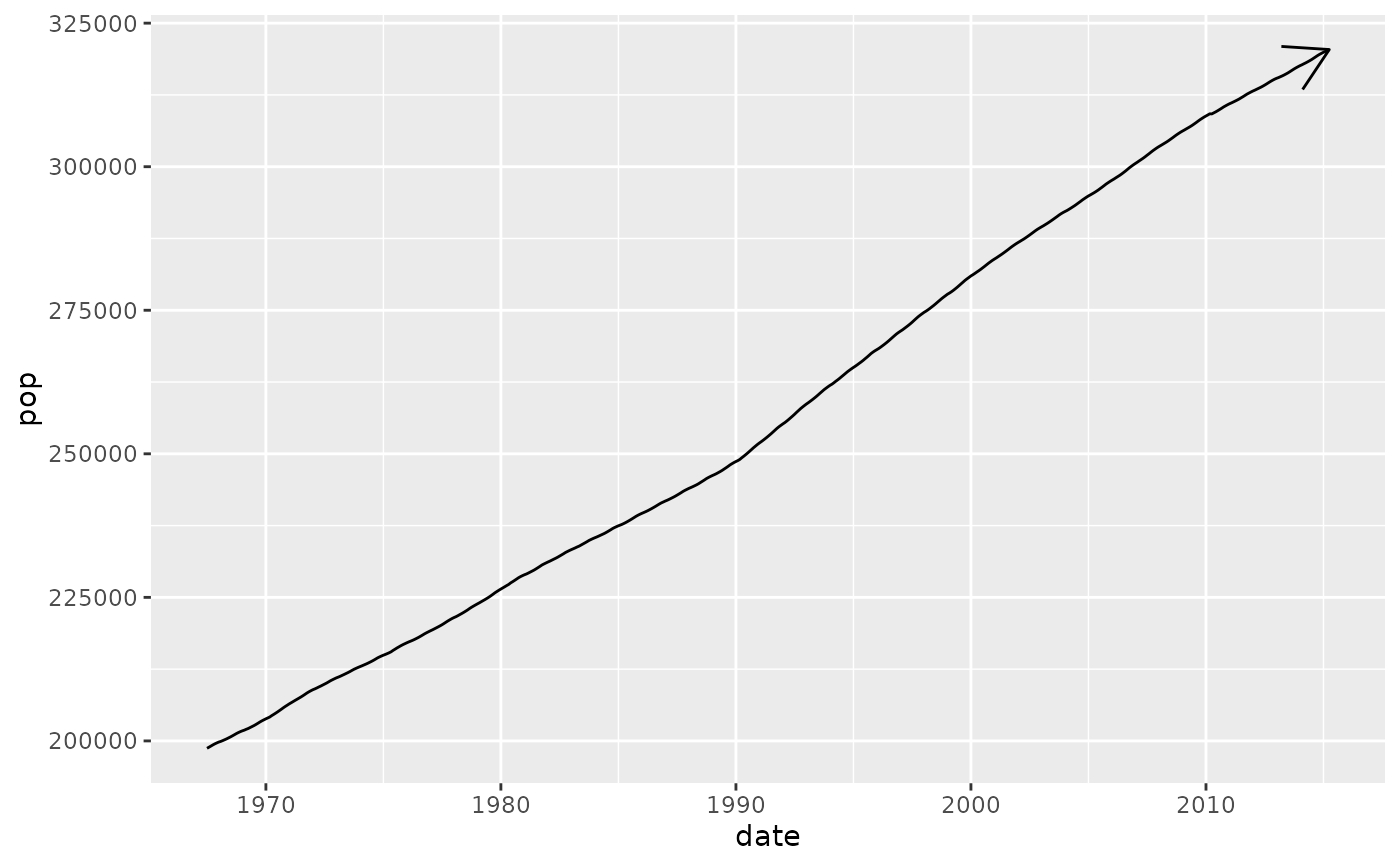
 # Use the arrow parameter to add an arrow to the line
# See ?arrow for more details
c <- ggplot(economics, aes(x = date, y = pop))
c + geom_line(arrow = arrow())
# Use the arrow parameter to add an arrow to the line
# See ?arrow for more details
c <- ggplot(economics, aes(x = date, y = pop))
c + geom_line(arrow = arrow())
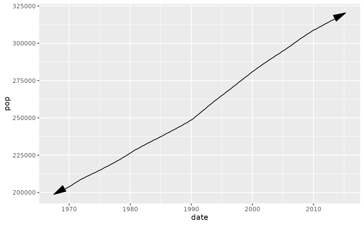
 c + geom_line(
arrow = arrow(angle = 15, ends = "both", type = "closed")
)
c + geom_line(
arrow = arrow(angle = 15, ends = "both", type = "closed")
)
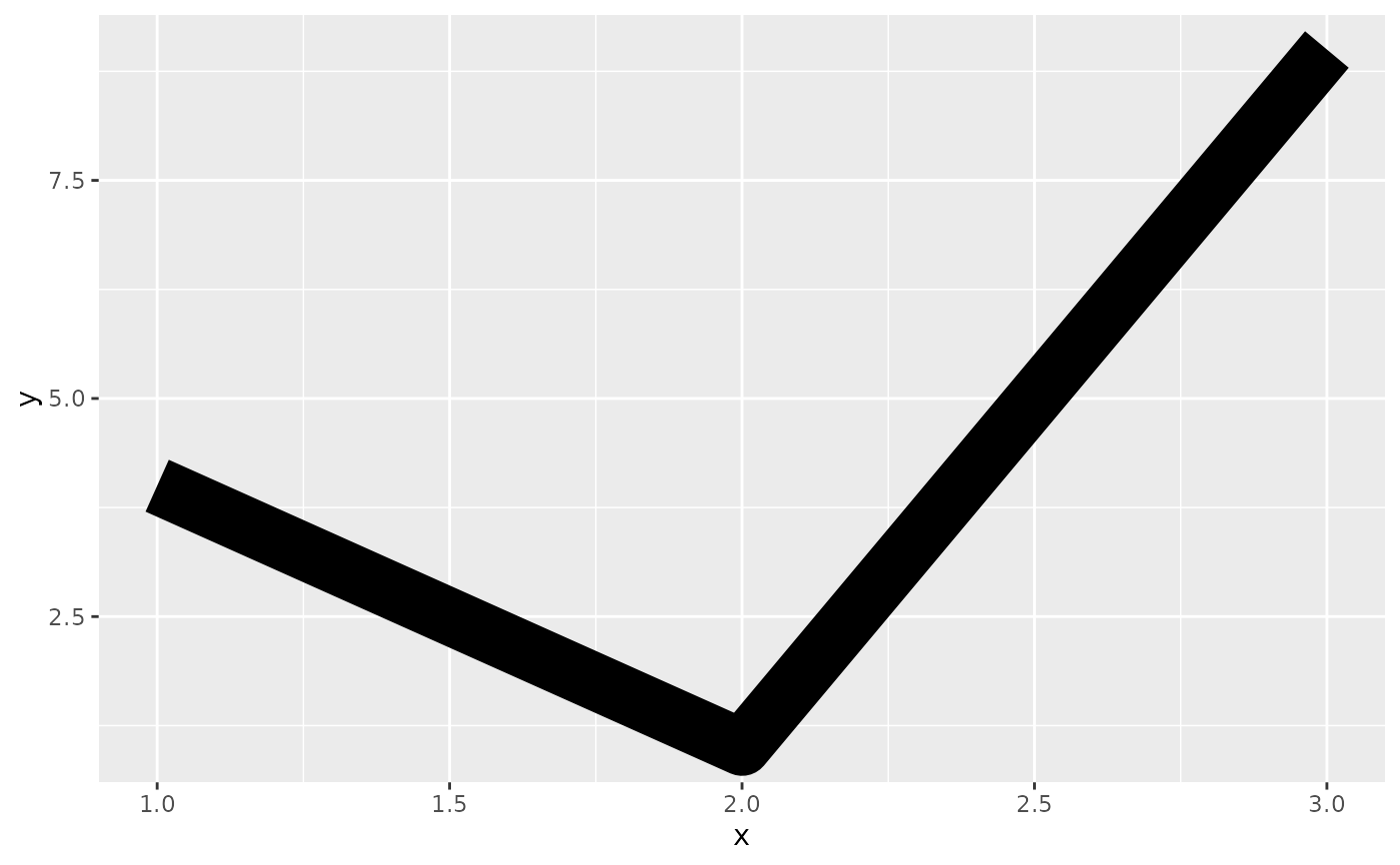
 # Control line join parameters
df <- data.frame(x = 1:3, y = c(4, 1, 9))
base <- ggplot(df, aes(x, y))
base + geom_path(linewidth = 10)
# Control line join parameters
df <- data.frame(x = 1:3, y = c(4, 1, 9))
base <- ggplot(df, aes(x, y))
base + geom_path(linewidth = 10)
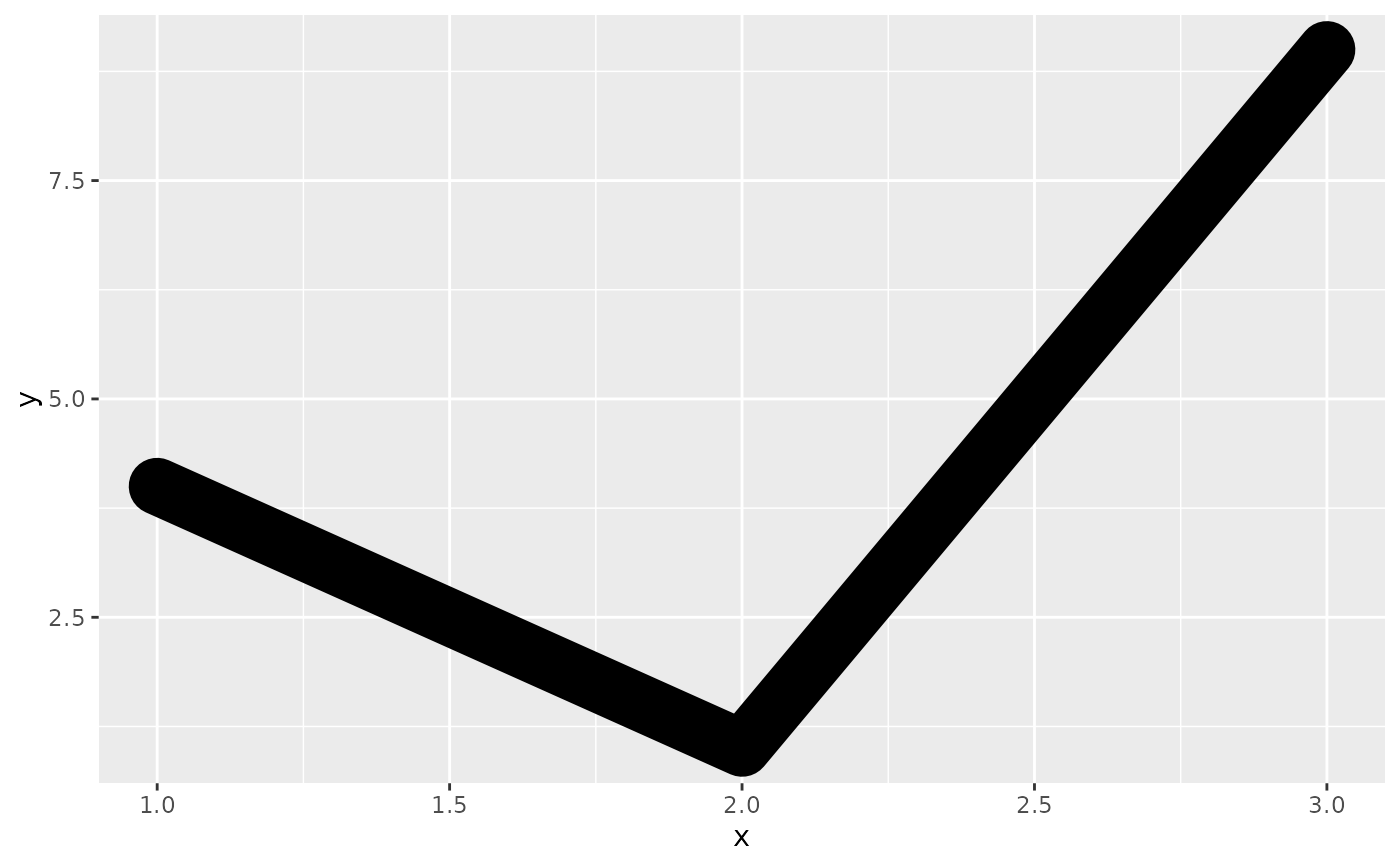
 base + geom_path(linewidth = 10, lineend = "round")
 base + geom_path(linewidth = 10, linejoin = "mitre", lineend = "butt")
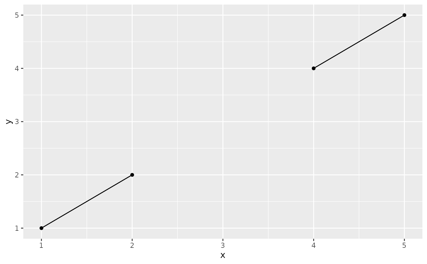
 # You can use NAs to break the line.
df <- data.frame(x = 1:5, y = c(1, 2, NA, 4, 5))
ggplot(df, aes(x, y)) + geom_point() + geom_line()
#> Warning: Removed 1 row containing missing values or values outside the scale
#> range (`geom_point()`).
# You can use NAs to break the line.
df <- data.frame(x = 1:5, y = c(1, 2, NA, 4, 5))
ggplot(df, aes(x, y)) + geom_point() + geom_line()
#> Warning: Removed 1 row containing missing values or values outside the scale
#> range (`geom_point()`).
 # \donttest{
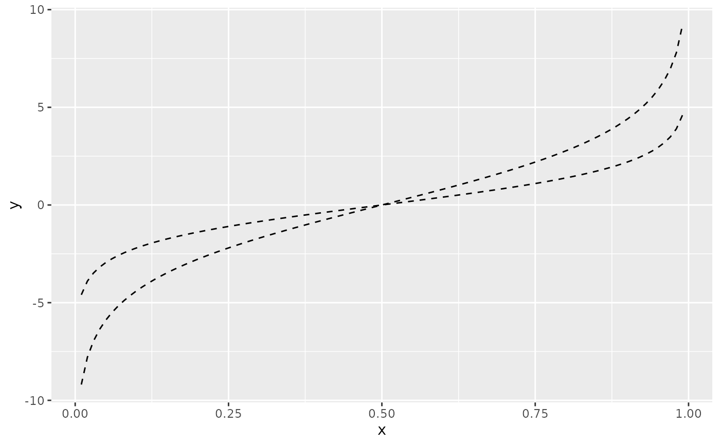
# Setting line type vs colour/size
# Line type needs to be applied to a line as a whole, so it can
# not be used with colour or size that vary across a line
x <- seq(0.01, .99, length.out = 100)
df <- data.frame(
x = rep(x, 2),
y = c(qlogis(x), 2 * qlogis(x)),
group = rep(c("a","b"),
each = 100)
)
p <- ggplot(df, aes(x=x, y=y, group=group))
# These work
p + geom_line(linetype = 2)
# \donttest{
# Setting line type vs colour/size
# Line type needs to be applied to a line as a whole, so it can
# not be used with colour or size that vary across a line
x <- seq(0.01, .99, length.out = 100)
df <- data.frame(
x = rep(x, 2),
y = c(qlogis(x), 2 * qlogis(x)),
group = rep(c("a","b"),
each = 100)
)
p <- ggplot(df, aes(x=x, y=y, group=group))
# These work
p + geom_line(linetype = 2)
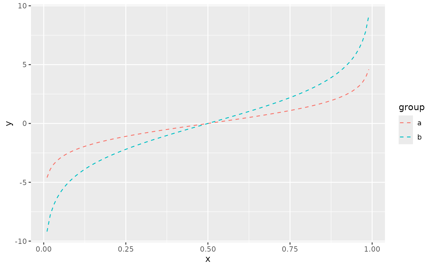
 p + geom_line(aes(colour = group), linetype = 2)
 p + geom_line(aes(colour = x))
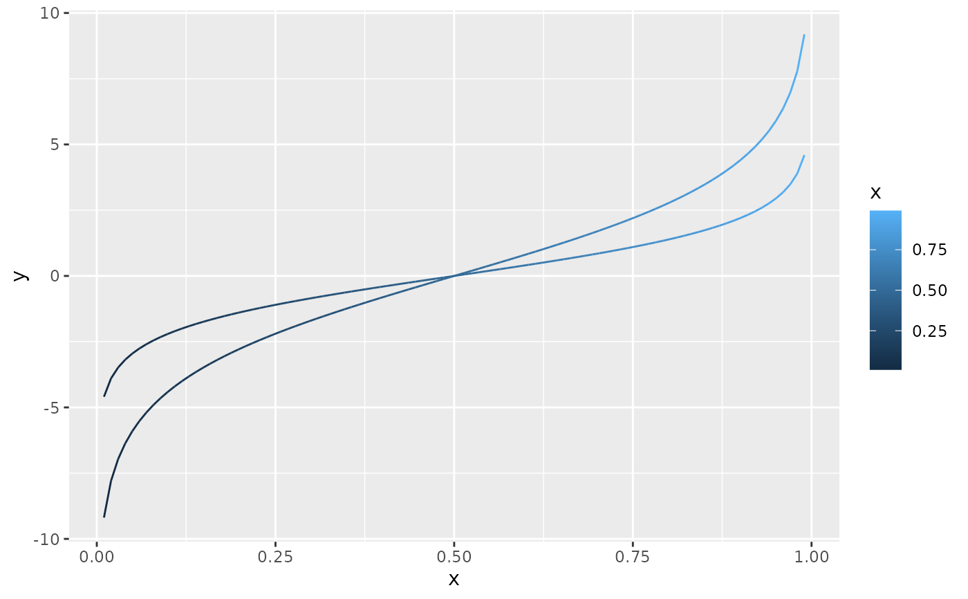 # But this doesn't
should_stop(p + geom_line(aes(colour = x), linetype=2))
# }
# But this doesn't
should_stop(p + geom_line(aes(colour = x), linetype=2))
# }