There are two types of bar charts: geom_bar() and geom_col().
geom_bar() makes the height of the bar proportional to the number of
cases in each group (or if the weight aesthetic is supplied, the sum
of the weights). If you want the heights of the bars to represent values
in the data, use geom_col() instead. geom_bar() uses stat_count() by
default: it counts the number of cases at each x position. geom_col()
uses stat_identity(): it leaves the data as is.
Usage
geom_bar(
  mapping = NULL,
  data = NULL,
  stat = "count",
  position = "stack",
  ...,
  just = 0.5,
  lineend = "butt",
  linejoin = "mitre",
  na.rm = FALSE,
  show.legend = NA,
  inherit.aes = TRUE
)

geom_col(
  mapping = NULL,
  data = NULL,
  stat = "identity",
  position = "stack",
  ...,
  just = 0.5,
  lineend = "butt",
  linejoin = "mitre",
  na.rm = FALSE,
  show.legend = NA,
  inherit.aes = TRUE
)

stat_count(
  mapping = NULL,
  data = NULL,
  geom = "bar",
  position = "stack",
  ...,
  orientation = NA,
  na.rm = FALSE,
  show.legend = NA,
  inherit.aes = TRUE
)
Arguments
- mapping
Set of aesthetic mappings created by
aes(). If specified andinherit.aes = TRUE(the default), it is combined with the default mapping at the top level of the plot. You must supplymappingif there is no plot mapping.- data
The data to be displayed in this layer. There are three options:
If
NULL, the default, the data is inherited from the plot data as specified in the call toggplot().A
data.frame, or other object, will override the plot data. All objects will be fortified to produce a data frame. Seefortify()for which variables will be created.A
functionwill be called with a single argument, the plot data. The return value must be adata.frame, and will be used as the layer data. Afunctioncan be created from aformula(e.g.~ head(.x, 10)).- position
A position adjustment to use on the data for this layer. This can be used in various ways, including to prevent overplotting and improving the display. The
positionargument accepts the following:The result of calling a position function, such as
position_jitter(). This method allows for passing extra arguments to the position.A string naming the position adjustment. To give the position as a string, strip the function name of the
position_prefix. For example, to useposition_jitter(), give the position as"jitter".For more information and other ways to specify the position, see the layer position documentation.
- ...
Other arguments passed on to
layer()'sparamsargument. These arguments broadly fall into one of 4 categories below. Notably, further arguments to thepositionargument, or aesthetics that are required can not be passed through.... Unknown arguments that are not part of the 4 categories below are ignored.Static aesthetics that are not mapped to a scale, but are at a fixed value and apply to the layer as a whole. For example,
colour = "red"orlinewidth = 3. The geom's documentation has an Aesthetics section that lists the available options. The 'required' aesthetics cannot be passed on to theparams. Please note that while passing unmapped aesthetics as vectors is technically possible, the order and required length is not guaranteed to be parallel to the input data.When constructing a layer using a
stat_*()function, the...argument can be used to pass on parameters to thegeompart of the layer. An example of this isstat_density(geom = "area", outline.type = "both"). The geom's documentation lists which parameters it can accept.Inversely, when constructing a layer using a
geom_*()function, the...argument can be used to pass on parameters to thestatpart of the layer. An example of this isgeom_area(stat = "density", adjust = 0.5). The stat's documentation lists which parameters it can accept.The
key_glyphargument oflayer()may also be passed on through.... This can be one of the functions described as key glyphs, to change the display of the layer in the legend.
- just
Adjustment for column placement. Set to
0.5by default, meaning that columns will be centered about axis breaks. Set to0or1to place columns to the left/right of axis breaks. Note that this argument may have unintended behaviour when used with alternative positions, e.g.position_dodge().- lineend
Line end style (round, butt, square).
- linejoin
Line join style (round, mitre, bevel).
- na.rm
If
FALSE, the default, missing values are removed with a warning. IfTRUE, missing values are silently removed.- show.legend
logical. Should this layer be included in the legends?
NA, the default, includes if any aesthetics are mapped.FALSEnever includes, andTRUEalways includes. It can also be a named logical vector to finely select the aesthetics to display. To include legend keys for all levels, even when no data exists, useTRUE. IfNA, all levels are shown in legend, but unobserved levels are omitted.- inherit.aes
If
FALSE, overrides the default aesthetics, rather than combining with them. This is most useful for helper functions that define both data and aesthetics and shouldn't inherit behaviour from the default plot specification, e.g.annotation_borders().- geom, stat
Override the default connection between
geom_bar()andstat_count(). For more information about overriding these connections, see how the stat and geom arguments work.- orientation
The orientation of the layer. The default (
NA) automatically determines the orientation from the aesthetic mapping. In the rare event that this fails it can be given explicitly by settingorientationto either"x"or"y". See the Orientation section for more detail.
Details
A bar chart uses height to represent a value, and so the base of the
bar must always be shown to produce a valid visual comparison.
Proceed with caution when using transformed scales with a bar chart.
It's important to always use a meaningful reference point for the base of the bar.
For example, for log transformations the reference point is 1. In fact, when
using a log scale, geom_bar() automatically places the base of the bar at 1.
Furthermore, never use stacked bars with a transformed scale, because scaling
happens before stacking. As a consequence, the height of bars will be wrong
when stacking occurs with a transformed scale.
By default, multiple bars occupying the same x position will be stacked
atop one another by position_stack(). If you want them to be dodged
side-to-side, use position_dodge() or position_dodge2(). Finally,
position_fill() shows relative proportions at each x by stacking the
bars and then standardising each bar to have the same height.
Orientation
This geom treats each axis differently and, thus, can thus have two orientations. Often the orientation is easy to deduce from a combination of the given mappings and the types of positional scales in use. Thus, ggplot2 will by default try to guess which orientation the layer should have. Under rare circumstances, the orientation is ambiguous and guessing may fail. In that case the orientation can be specified directly using the orientation parameter, which can be either "x" or "y". The value gives the axis that the geom should run along, "x" being the default orientation you would expect for the geom.
Computed variables
These are calculated by the 'stat' part of layers and can be accessed with delayed evaluation.
after_stat(count)
number of points in bin.after_stat(prop)
groupwise proportion
See also
geom_histogram() for continuous data,
position_dodge() and position_dodge2() for creating side-by-side
bar charts.
stat_bin(), which bins data in ranges and counts the
cases in each range. It differs from stat_count(), which counts the
number of cases at each x position (without binning into ranges).
stat_bin() requires continuous x data, whereas
stat_count() can be used for both discrete and continuous x data.
Aesthetics
geom_bar() understands the following aesthetics. Required aesthetics are displayed in bold and defaults are displayed for optional aesthetics:
| • | x | |
| • | y | |
| • | alpha | → NA |
| • | colour | → via theme() |
| • | fill | → via theme() |
| • | group | → inferred |
| • | linetype | → via theme() |
| • | linewidth | → via theme() |
| • | width | → 0.9 |
geom_col() understands the following aesthetics. Required aesthetics are displayed in bold and defaults are displayed for optional aesthetics:
| • | x | |
| • | y | |
| • | alpha | → NA |
| • | colour | → via theme() |
| • | fill | → via theme() |
| • | group | → inferred |
| • | linetype | → via theme() |
| • | linewidth | → via theme() |
| • | width | → 0.9 |
stat_count() understands the following aesthetics. Required aesthetics are displayed in bold and defaults are displayed for optional aesthetics:
| • | x or y | |
| • | group | → inferred |
| • | weight | → 1 |
Learn more about setting these aesthetics in vignette("ggplot2-specs").
Examples
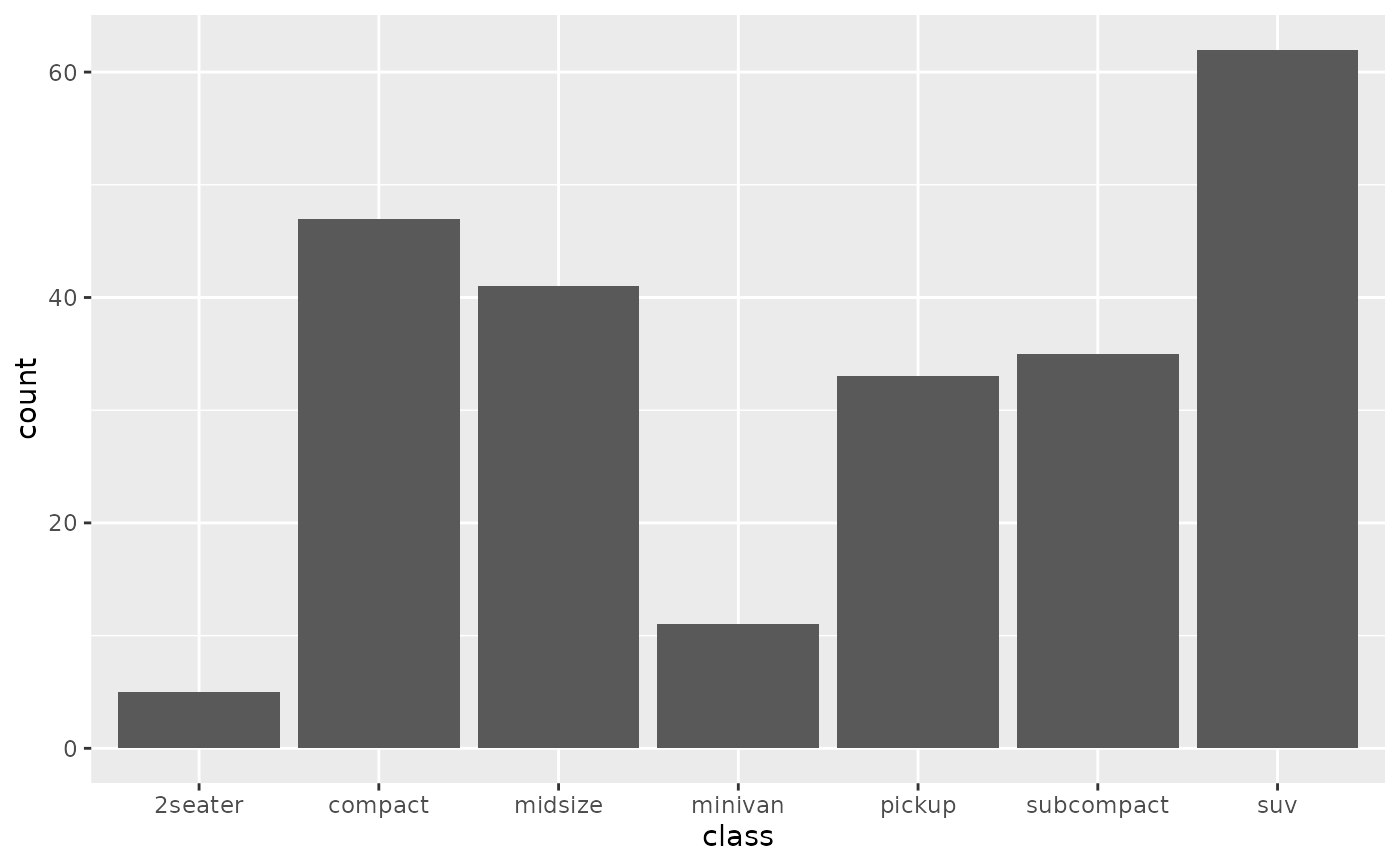
# geom_bar is designed to make it easy to create bar charts that show
# counts (or sums of weights)
g <- ggplot(mpg, aes(class))
# Number of cars in each class:
g + geom_bar()
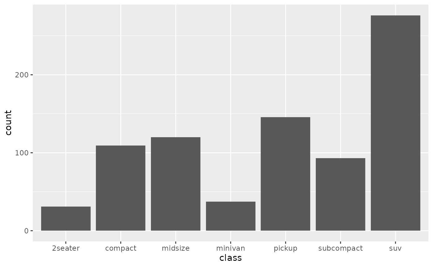
 # Total engine displacement of each class
g + geom_bar(aes(weight = displ))
# Total engine displacement of each class
g + geom_bar(aes(weight = displ))
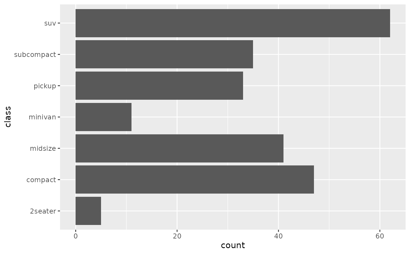
 # Map class to y instead to flip the orientation
ggplot(mpg) + geom_bar(aes(y = class))
# Map class to y instead to flip the orientation
ggplot(mpg) + geom_bar(aes(y = class))
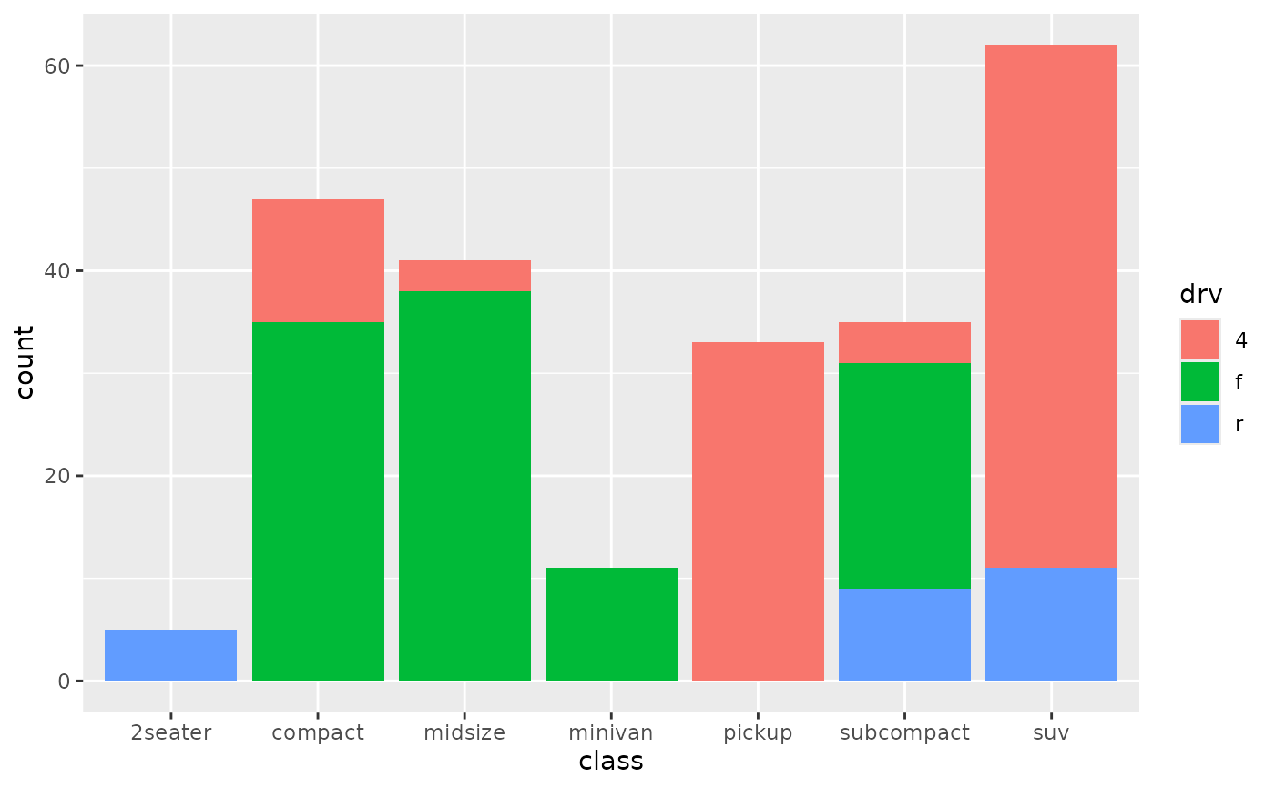
 # Bar charts are automatically stacked when multiple bars are placed
# at the same location. The order of the fill is designed to match
# the legend
g + geom_bar(aes(fill = drv))
# Bar charts are automatically stacked when multiple bars are placed
# at the same location. The order of the fill is designed to match
# the legend
g + geom_bar(aes(fill = drv))
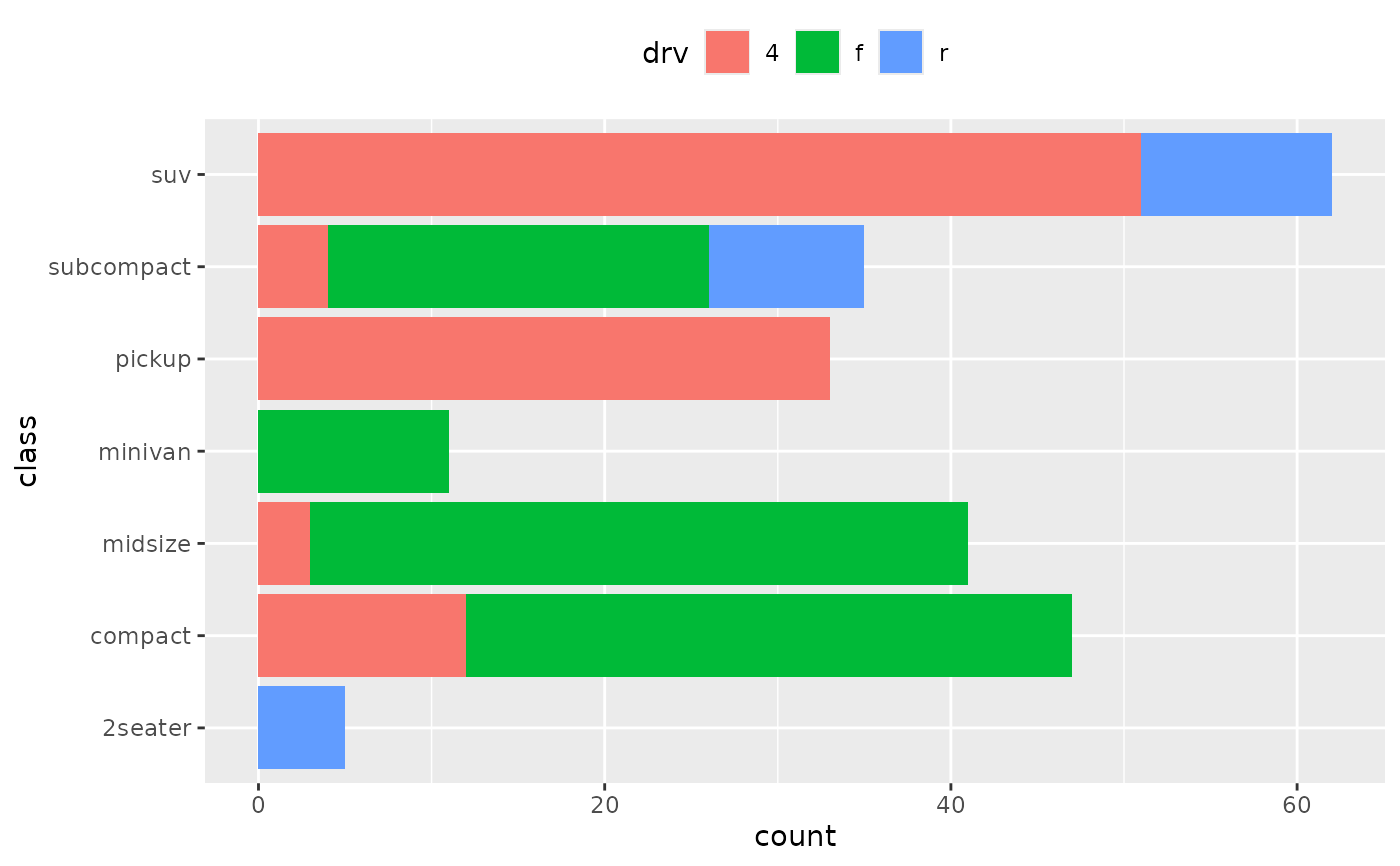
 # If you need to flip the order (because you've flipped the orientation)
# call position_stack() explicitly:
ggplot(mpg, aes(y = class)) +
geom_bar(aes(fill = drv), position = position_stack(reverse = TRUE)) +
theme(legend.position = "top")
# If you need to flip the order (because you've flipped the orientation)
# call position_stack() explicitly:
ggplot(mpg, aes(y = class)) +
geom_bar(aes(fill = drv), position = position_stack(reverse = TRUE)) +
theme(legend.position = "top")
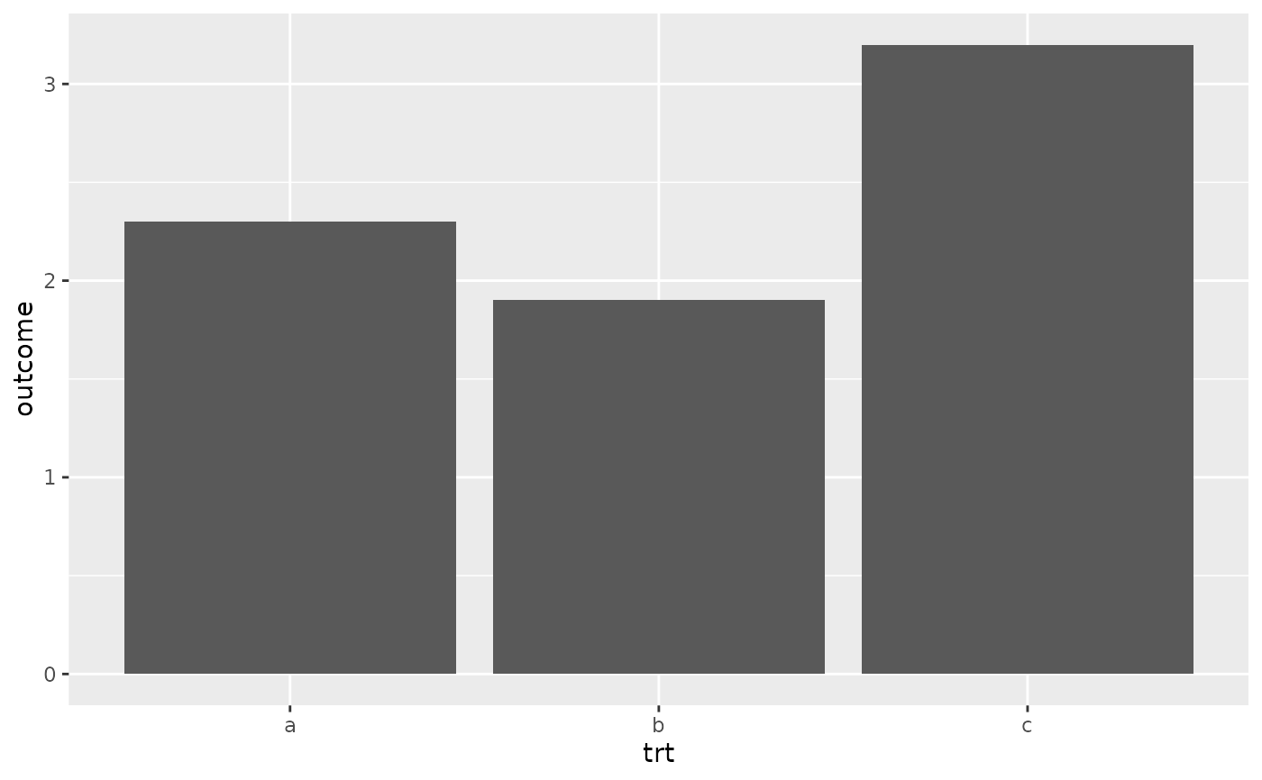
 # To show (e.g.) means, you need geom_col()
df <- data.frame(trt = c("a", "b", "c"), outcome = c(2.3, 1.9, 3.2))
ggplot(df, aes(trt, outcome)) +
geom_col()
# To show (e.g.) means, you need geom_col()
df <- data.frame(trt = c("a", "b", "c"), outcome = c(2.3, 1.9, 3.2))
ggplot(df, aes(trt, outcome)) +
geom_col()
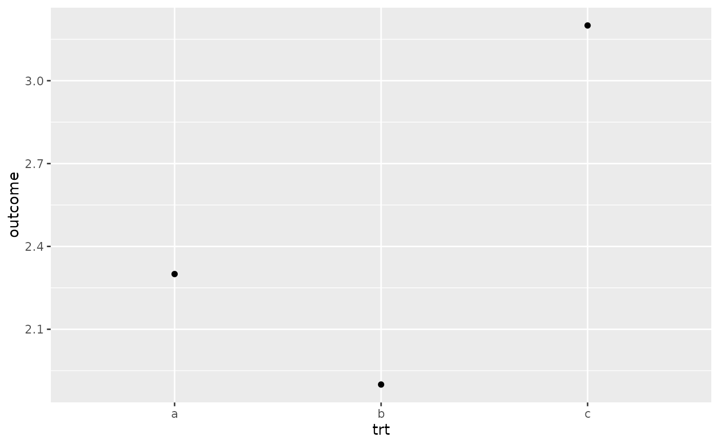
 # But geom_point() displays exactly the same information and doesn't
# require the y-axis to touch zero.
ggplot(df, aes(trt, outcome)) +
geom_point()
# But geom_point() displays exactly the same information and doesn't
# require the y-axis to touch zero.
ggplot(df, aes(trt, outcome)) +
geom_point()
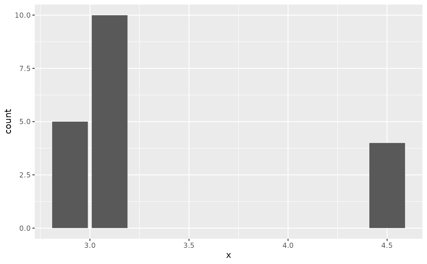
 # You can also use geom_bar() with continuous data, in which case
# it will show counts at unique locations
df <- data.frame(x = rep(c(2.9, 3.1, 4.5), c(5, 10, 4)))
ggplot(df, aes(x)) + geom_bar()
# You can also use geom_bar() with continuous data, in which case
# it will show counts at unique locations
df <- data.frame(x = rep(c(2.9, 3.1, 4.5), c(5, 10, 4)))
ggplot(df, aes(x)) + geom_bar()
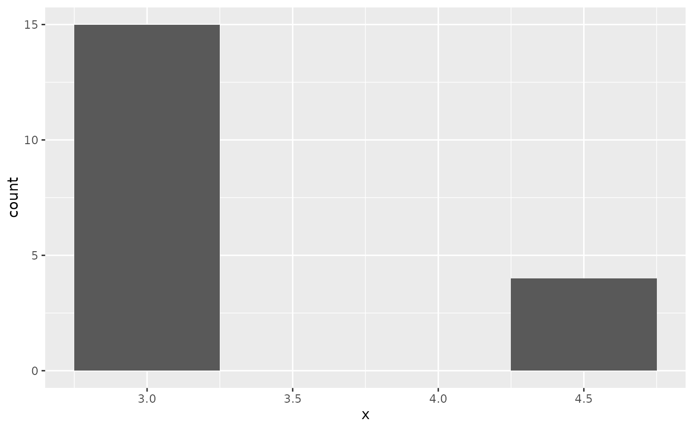
 # cf. a histogram of the same data
ggplot(df, aes(x)) + geom_histogram(binwidth = 0.5)
# cf. a histogram of the same data
ggplot(df, aes(x)) + geom_histogram(binwidth = 0.5)
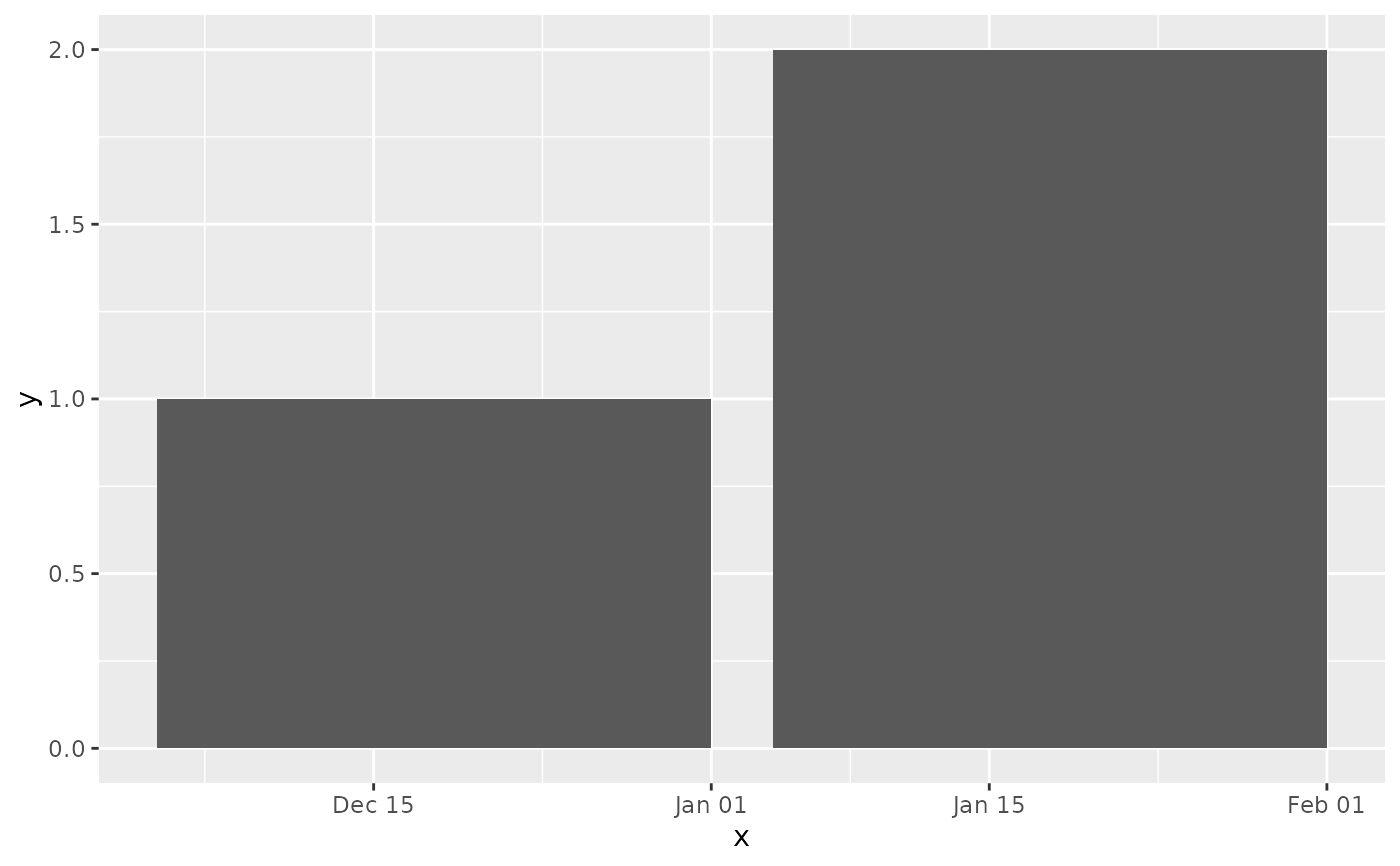
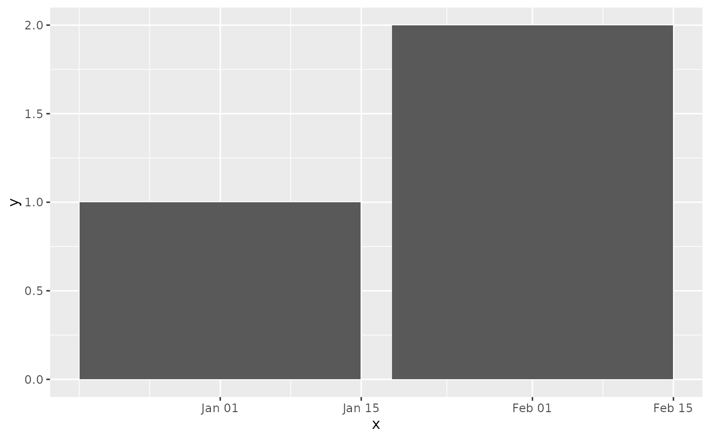
 # Use `just` to control how columns are aligned with axis breaks:
df <- data.frame(x = as.Date(c("2020-01-01", "2020-02-01")), y = 1:2)
# Columns centered on the first day of the month
ggplot(df, aes(x, y)) + geom_col(just = 0.5)
# Use `just` to control how columns are aligned with axis breaks:
df <- data.frame(x = as.Date(c("2020-01-01", "2020-02-01")), y = 1:2)
# Columns centered on the first day of the month
ggplot(df, aes(x, y)) + geom_col(just = 0.5)
 # Columns begin on the first day of the month
ggplot(df, aes(x, y)) + geom_col(just = 1)
# Columns begin on the first day of the month
ggplot(df, aes(x, y)) + geom_col(just = 1)