This is a shortcut for supplying the limits argument to the individual
scales. By default, any values outside the limits specified are replaced with
NA. Be warned that this will remove data outside the limits and this can
produce unintended results. For changing x or y axis limits without
dropping data observations, see
coord_cartesian(xlim, ylim), or use a full scale with
oob = scales::oob_keep.
Arguments
- ...
For
xlim()andylim(): Two numeric values, specifying the left/lower limit and the right/upper limit of the scale. If the larger value is given first, the scale will be reversed. You can leave one value asNAif you want to compute the corresponding limit from the range of the data.For
lims(): A name–value pair. The name must be an aesthetic, and the value must be either a length-2 numeric, a character, a factor, or a date/time. A numeric value will create a continuous scale. If the larger value comes first, the scale will be reversed. You can leave one value asNAif you want to compute the corresponding limit from the range of the data. A character or factor value will create a discrete scale. A date-time value will create a continuous date/time scale.
See also
To expand the range of a plot to always include
certain values, see expand_limits(). For other types of data, see
scale_x_discrete(), scale_x_continuous(), scale_x_date().
Examples
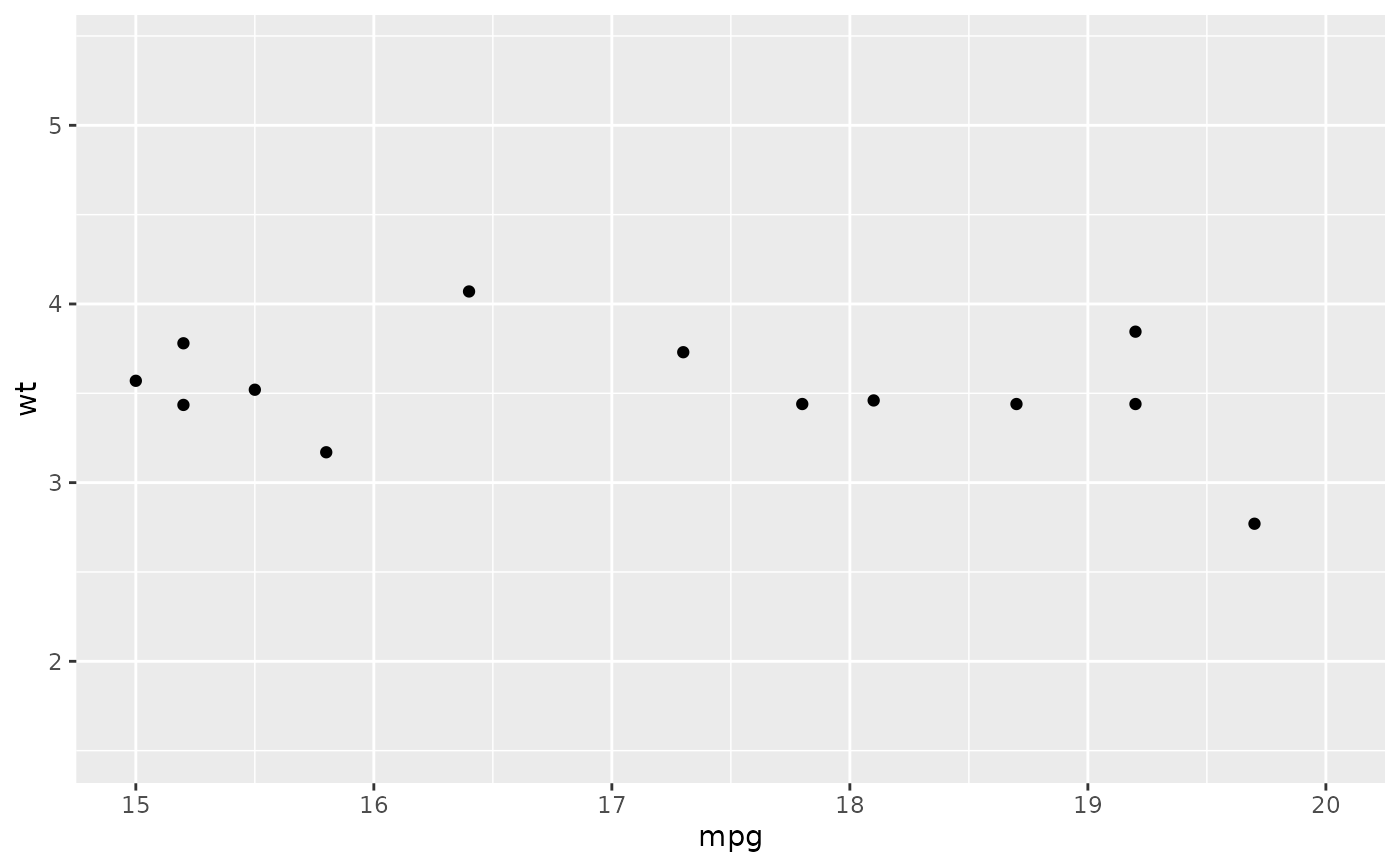
# Zoom into a specified area
ggplot(mtcars, aes(mpg, wt)) +
geom_point() +
xlim(15, 20)
#> Warning: Removed 19 rows containing missing values or values outside the scale
#> range (`geom_point()`).
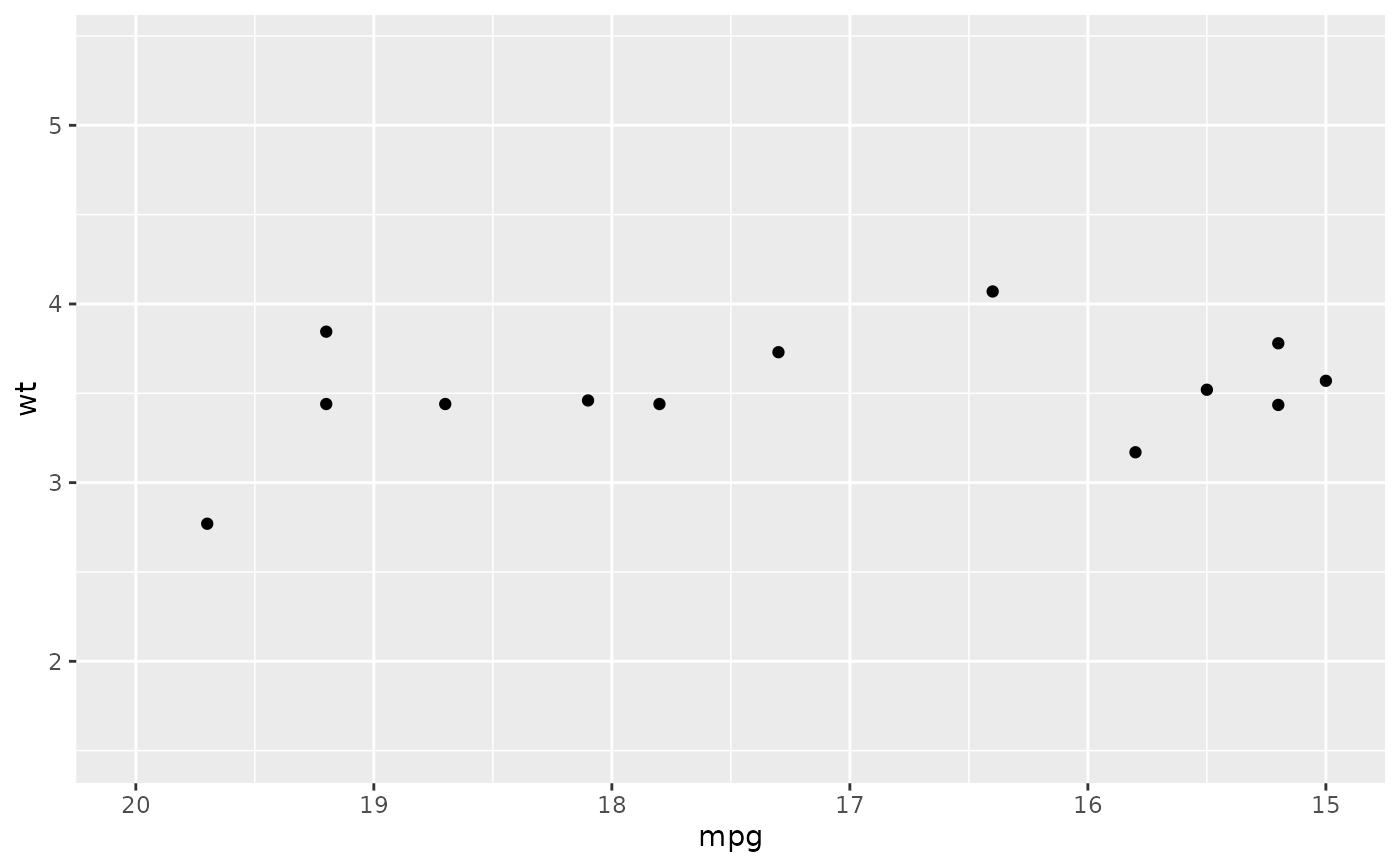
 # reverse scale
ggplot(mtcars, aes(mpg, wt)) +
geom_point() +
xlim(20, 15)
#> Warning: Removed 19 rows containing missing values or values outside the scale
#> range (`geom_point()`).
# reverse scale
ggplot(mtcars, aes(mpg, wt)) +
geom_point() +
xlim(20, 15)
#> Warning: Removed 19 rows containing missing values or values outside the scale
#> range (`geom_point()`).
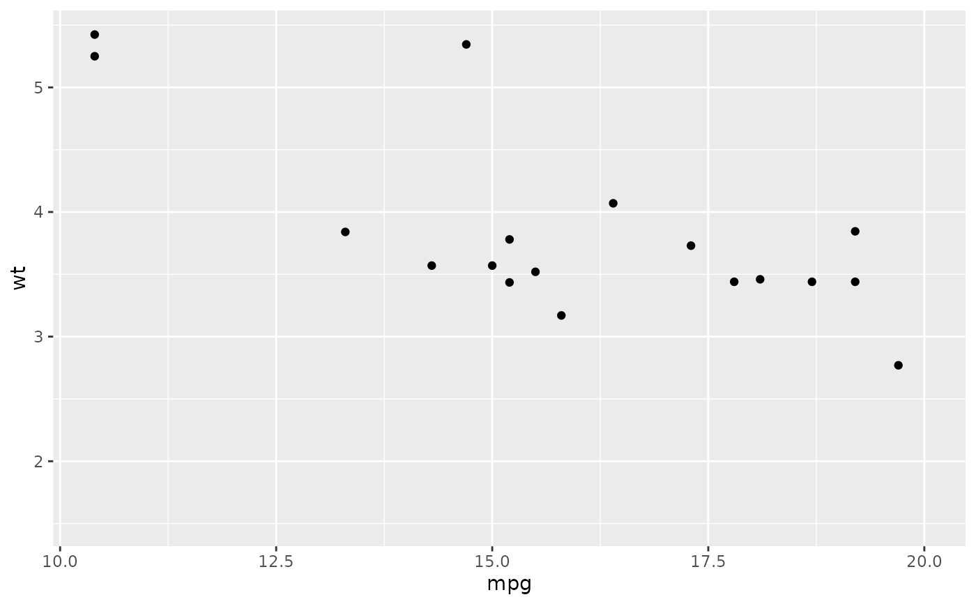
 # with automatic lower limit
ggplot(mtcars, aes(mpg, wt)) +
geom_point() +
xlim(NA, 20)
#> Warning: Removed 14 rows containing missing values or values outside the scale
#> range (`geom_point()`).
# with automatic lower limit
ggplot(mtcars, aes(mpg, wt)) +
geom_point() +
xlim(NA, 20)
#> Warning: Removed 14 rows containing missing values or values outside the scale
#> range (`geom_point()`).
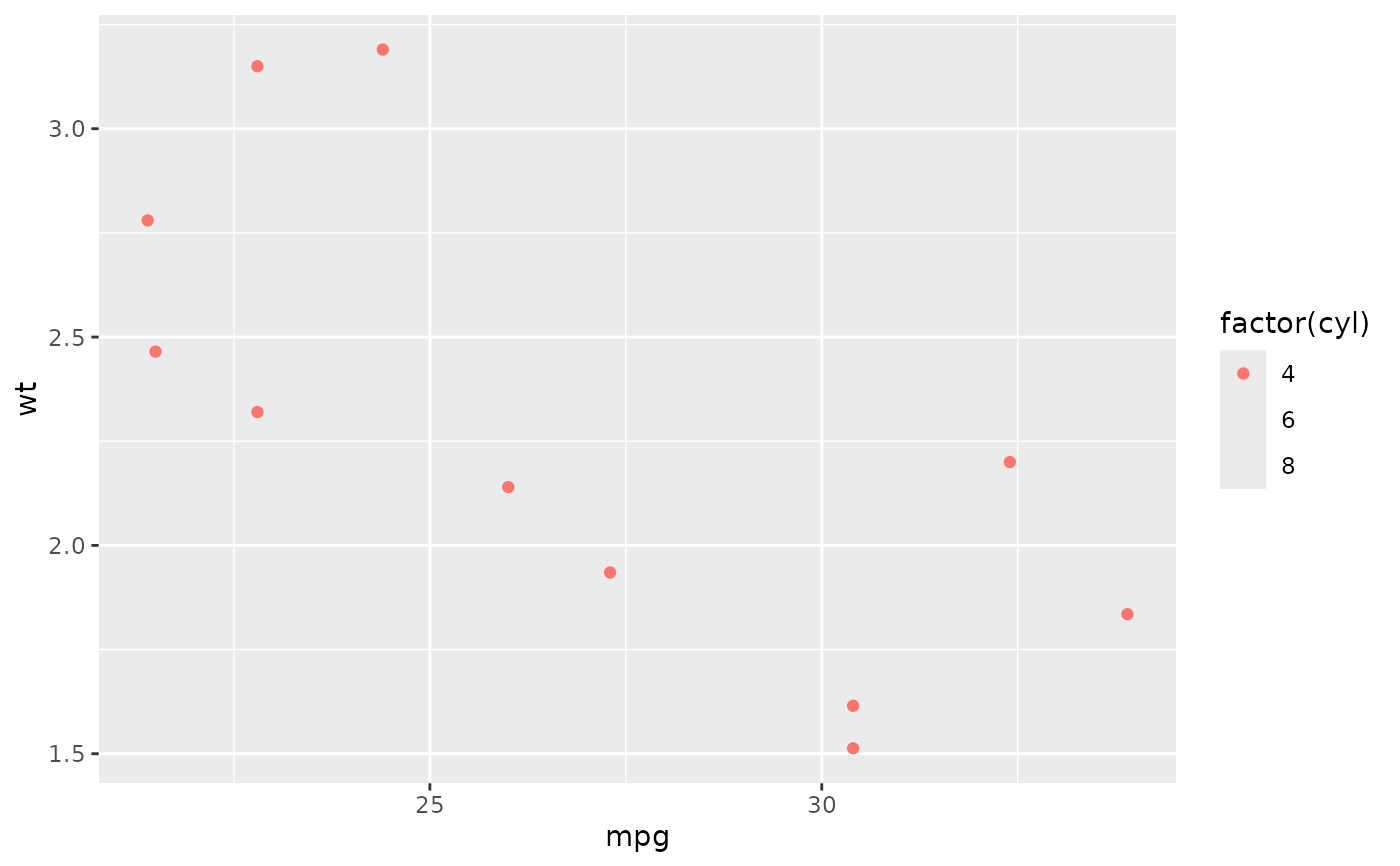
 # You can also supply limits that are larger than the data.
# This is useful if you want to match scales across different plots
small <- subset(mtcars, cyl == 4)
big <- subset(mtcars, cyl > 4)
ggplot(small, aes(mpg, wt, colour = factor(cyl))) +
geom_point() +
lims(colour = c("4", "6", "8"))
# You can also supply limits that are larger than the data.
# This is useful if you want to match scales across different plots
small <- subset(mtcars, cyl == 4)
big <- subset(mtcars, cyl > 4)
ggplot(small, aes(mpg, wt, colour = factor(cyl))) +
geom_point() +
lims(colour = c("4", "6", "8"))
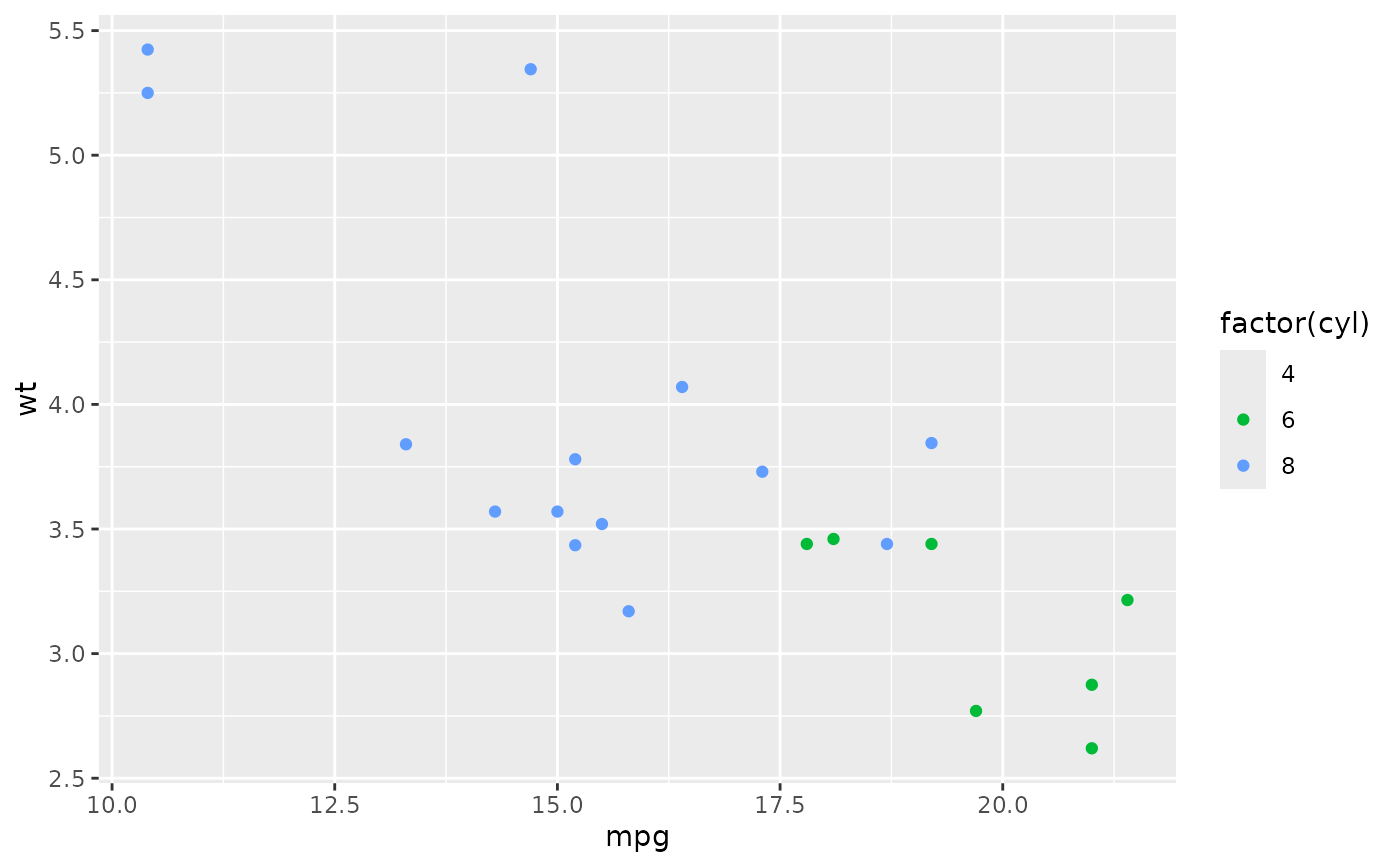
 ggplot(big, aes(mpg, wt, colour = factor(cyl))) +
geom_point() +
lims(colour = c("4", "6", "8"))
ggplot(big, aes(mpg, wt, colour = factor(cyl))) +
geom_point() +
lims(colour = c("4", "6", "8"))
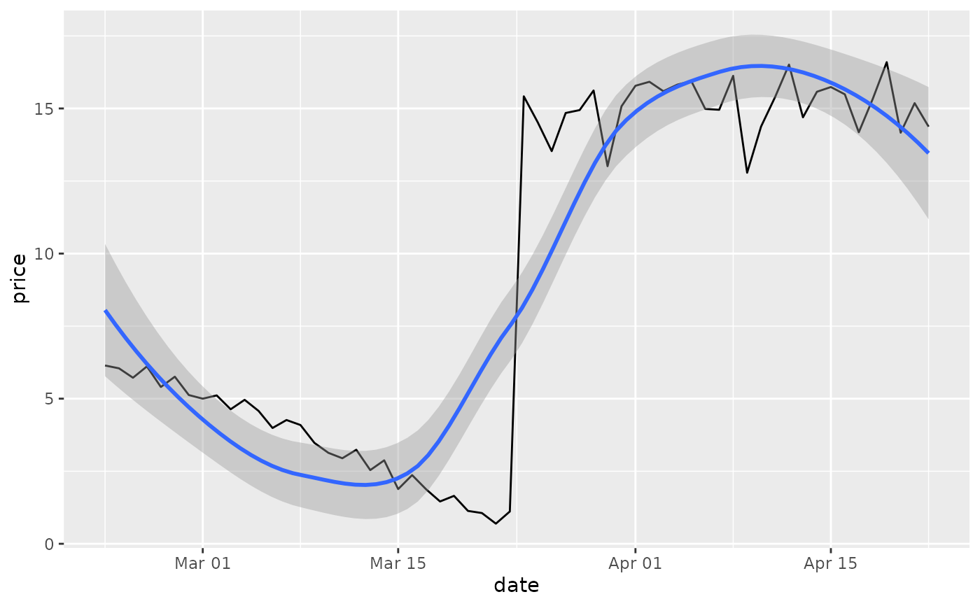
 # There are two ways of setting the axis limits: with limits or
# with coordinate systems. They work in two rather different ways.
set.seed(1)
last_month <- Sys.Date() - 0:59
df <- data.frame(
date = last_month,
price = c(rnorm(30, mean = 15), runif(30) + 0.2 * (1:30))
)
p <- ggplot(df, aes(date, price)) +
geom_line() +
stat_smooth()
p
#> `geom_smooth()` using method = 'loess' and formula = 'y ~ x'
# There are two ways of setting the axis limits: with limits or
# with coordinate systems. They work in two rather different ways.
set.seed(1)
last_month <- Sys.Date() - 0:59
df <- data.frame(
date = last_month,
price = c(rnorm(30, mean = 15), runif(30) + 0.2 * (1:30))
)
p <- ggplot(df, aes(date, price)) +
geom_line() +
stat_smooth()
p
#> `geom_smooth()` using method = 'loess' and formula = 'y ~ x'
 # Setting the limits with the scale discards all data outside the range.
p + lims(x= c(Sys.Date() - 30, NA), y = c(10, 20))
#> `geom_smooth()` using method = 'loess' and formula = 'y ~ x'
#> Warning: Removed 30 rows containing non-finite outside the scale range
#> (`stat_smooth()`).
#> Warning: Removed 30 rows containing missing values or values outside the scale
#> range (`geom_line()`).
# Setting the limits with the scale discards all data outside the range.
p + lims(x= c(Sys.Date() - 30, NA), y = c(10, 20))
#> `geom_smooth()` using method = 'loess' and formula = 'y ~ x'
#> Warning: Removed 30 rows containing non-finite outside the scale range
#> (`stat_smooth()`).
#> Warning: Removed 30 rows containing missing values or values outside the scale
#> range (`geom_line()`).
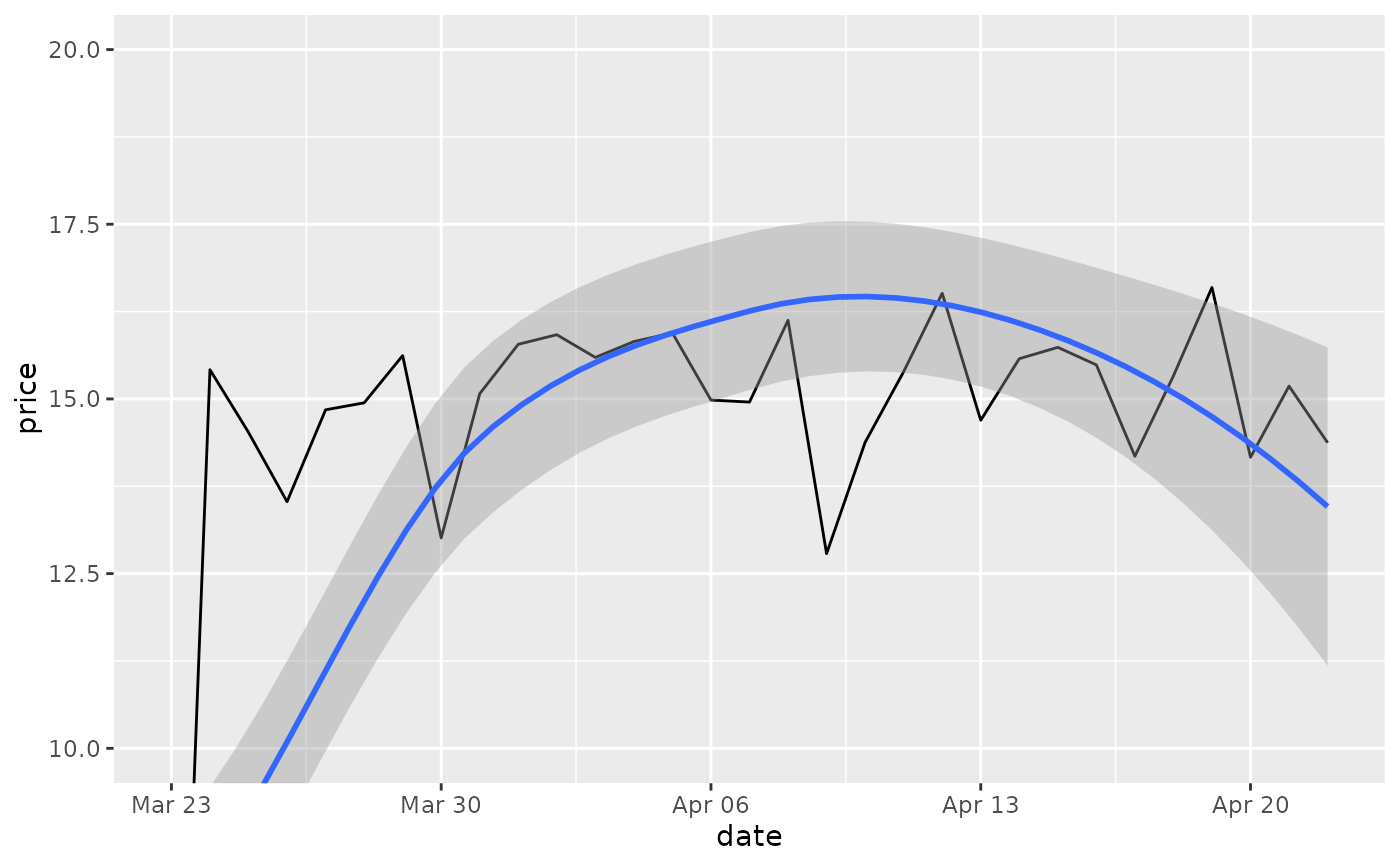
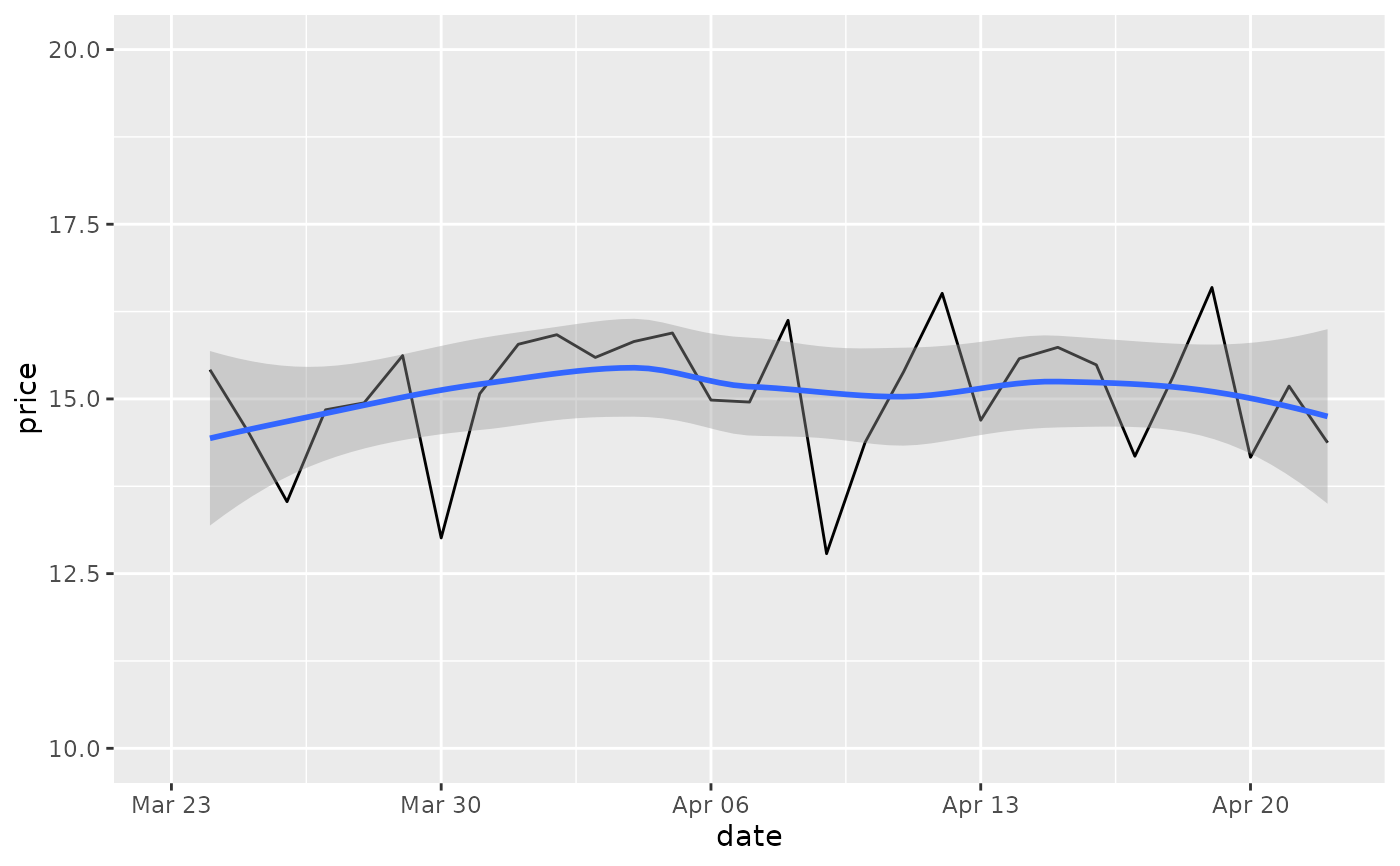 # For changing x or y axis limits **without** dropping data
# observations use [coord_cartesian()]. Setting the limits on the
# coordinate system performs a visual zoom.
p + coord_cartesian(xlim =c(Sys.Date() - 30, NA), ylim = c(10, 20))
#> `geom_smooth()` using method = 'loess' and formula = 'y ~ x'
# For changing x or y axis limits **without** dropping data
# observations use [coord_cartesian()]. Setting the limits on the
# coordinate system performs a visual zoom.
p + coord_cartesian(xlim =c(Sys.Date() - 30, NA), ylim = c(10, 20))
#> `geom_smooth()` using method = 'loess' and formula = 'y ~ x'