Cartesian coordinates

The Cartesian coordinate system is the most familiar, and common, type of coordinate system. Setting limits on the coordinate system will zoom the plot (like you're looking at it with a magnifying glass), and will not change the underlying data like setting limits on a scale will.

Usage

coord_cartesian(
  xlim = NULL,
  ylim = NULL,
  expand = TRUE,
  default = FALSE,
  clip = "on",
  reverse = "none"
)

Arguments

xlim, ylim

Limits for the x and y axes.

expand

If TRUE, the default, adds a small expansion factor to the limits to ensure that data and axes don't overlap. If FALSE, limits are taken exactly from the data or xlim/ylim. Giving a logical vector will separately control the expansion for the four directions (top, left, bottom and right). The expand argument will be recycled to length 4 if necessary. Alternatively, can be a named logical vector to control a single direction, e.g. expand = c(bottom = FALSE).

default

Is this the default coordinate system? If FALSE (the default), then replacing this coordinate system with another one creates a message alerting the user that the coordinate system is being replaced. If TRUE, that warning is suppressed.

clip

Should drawing be clipped to the extent of the plot panel? A setting of "on" (the default) means yes, and a setting of "off" means no. In most cases, the default of "on" should not be changed, as setting clip = "off" can cause unexpected results. It allows drawing of data points anywhere on the plot, including in the plot margins. If limits are set via xlim and ylim and some data points fall outside those limits, then those data points may show up in places such as the axes, the legend, the plot title, or the plot margins.

reverse

A string giving which directions to reverse. "none" (default) keeps directions as is. "x" and "y" can be used to reverse their respective directions. "xy" can be used to reverse both directions.

Examples

# There are two ways of zooming the plot display: with scales or
# with coordinate systems.  They work in two rather different ways.

p <- ggplot(mtcars, aes(disp, wt)) +
  geom_point() +
  geom_smooth()
p
#> `geom_smooth()` using method = 'loess' and formula = 'y ~ x'


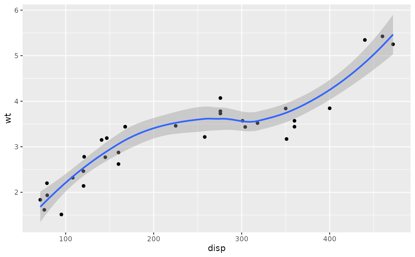# Setting the limits on a scale converts all values outside the range to NA.
p + scale_x_continuous(limits = c(325, 500))
#> `geom_smooth()` using method = 'loess' and formula = 'y ~ x'
#> Warning: Removed 24 rows containing non-finite outside the scale range
#> (`stat_smooth()`).
#> Warning: Removed 24 rows containing missing values or values outside the scale
#> range (`geom_point()`).


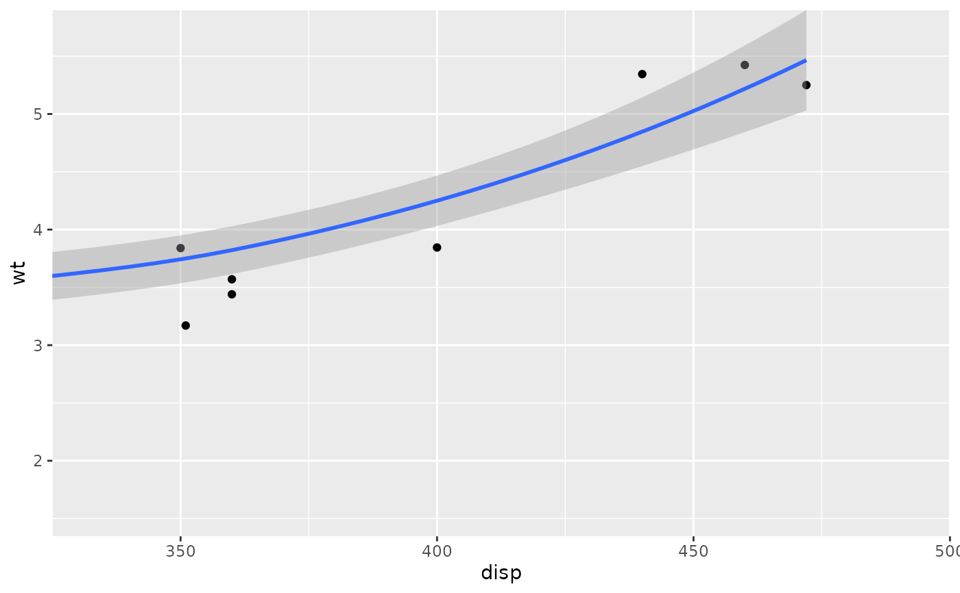
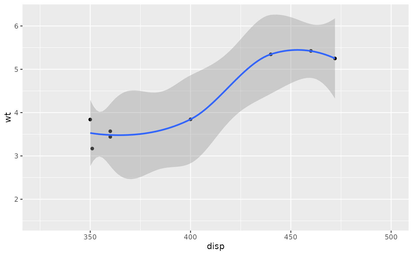# Setting the limits on the coordinate system performs a visual zoom.
# The data is unchanged, and we just view a small portion of the original
# plot. Note how smooth continues past the points visible on this plot.
p + coord_cartesian(xlim = c(325, 500))
#> `geom_smooth()` using method = 'loess' and formula = 'y ~ x'


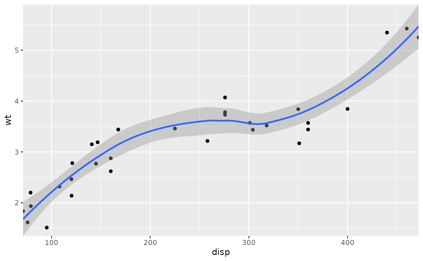
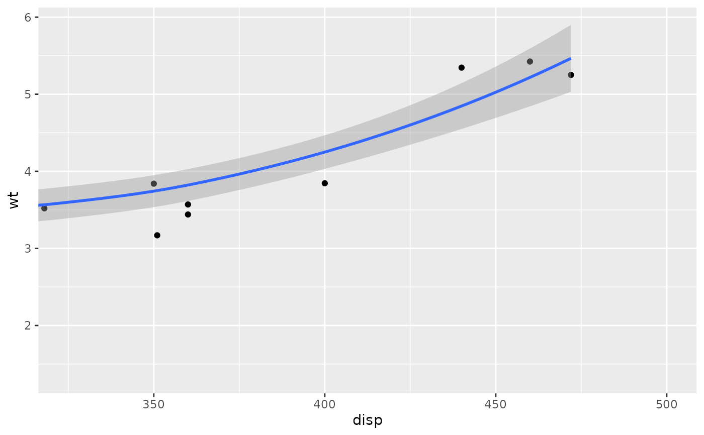# By default, the same expansion factor is applied as when setting scale
# limits. You can set the limits precisely by setting expand = FALSE
p + coord_cartesian(xlim = c(325, 500), expand = FALSE)
#> `geom_smooth()` using method = 'loess' and formula = 'y ~ x'


# Similarly, we can use expand = FALSE to turn off expansion with the
# default limits
p + coord_cartesian(expand = FALSE)
#> `geom_smooth()` using method = 'loess' and formula = 'y ~ x'


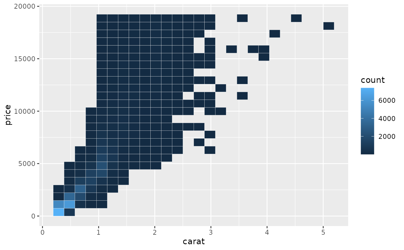# You can see the same thing with this 2d histogram
d <- ggplot(diamonds, aes(carat, price)) +
  stat_bin_2d(bins = 25, colour = "white")
d


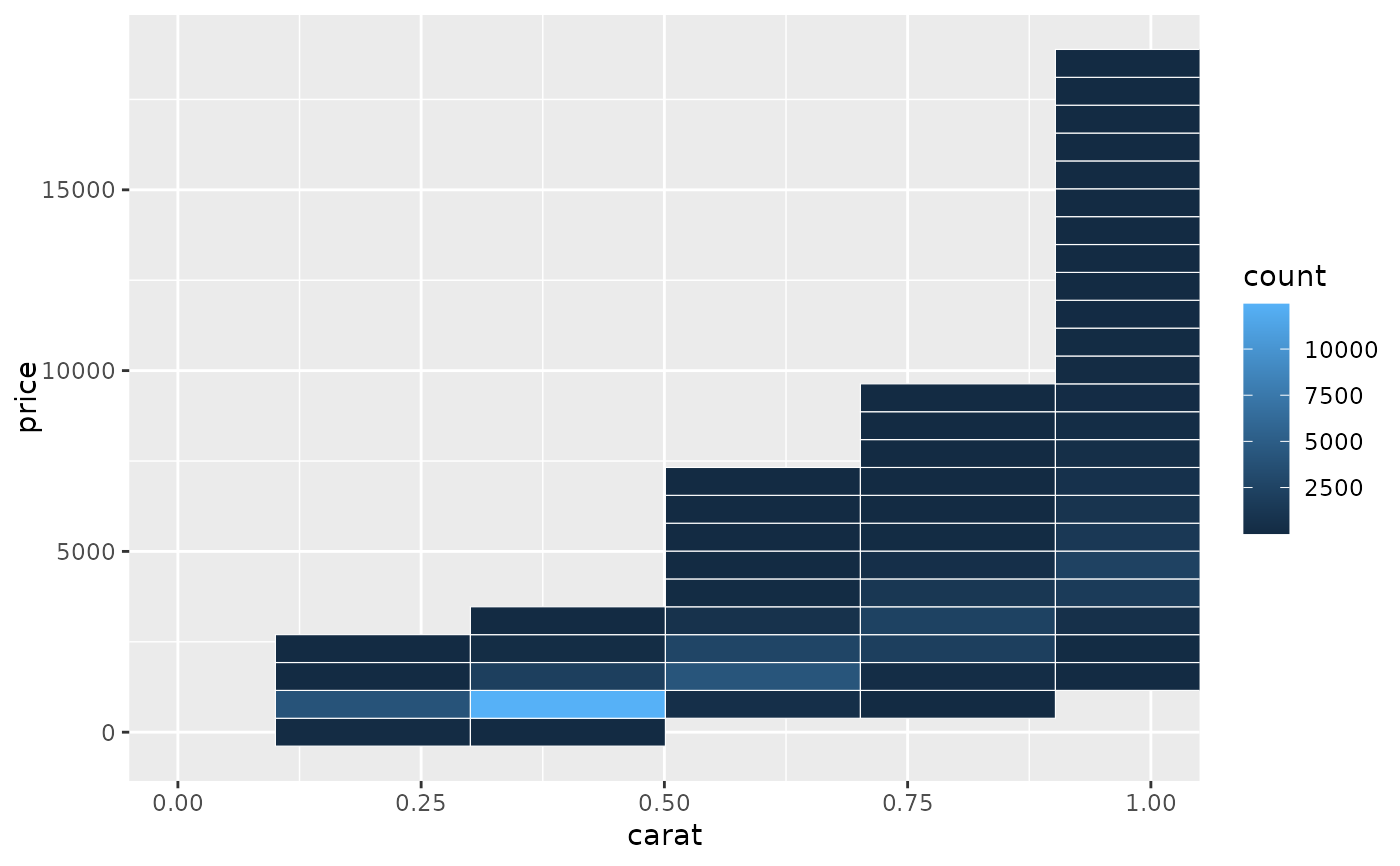
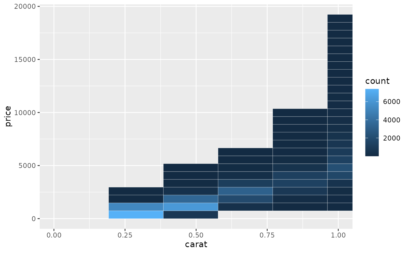
# When zooming the scale, the we get 25 new bins that are the same
# size on the plot, but represent smaller regions of the data space
d + scale_x_continuous(limits = c(0, 1))
#> Warning: Removed 17502 rows containing non-finite outside the scale range
#> (`stat_bin2d()`).
#> Warning: Removed 17 rows containing missing values or values outside the scale
#> range (`geom_tile()`).


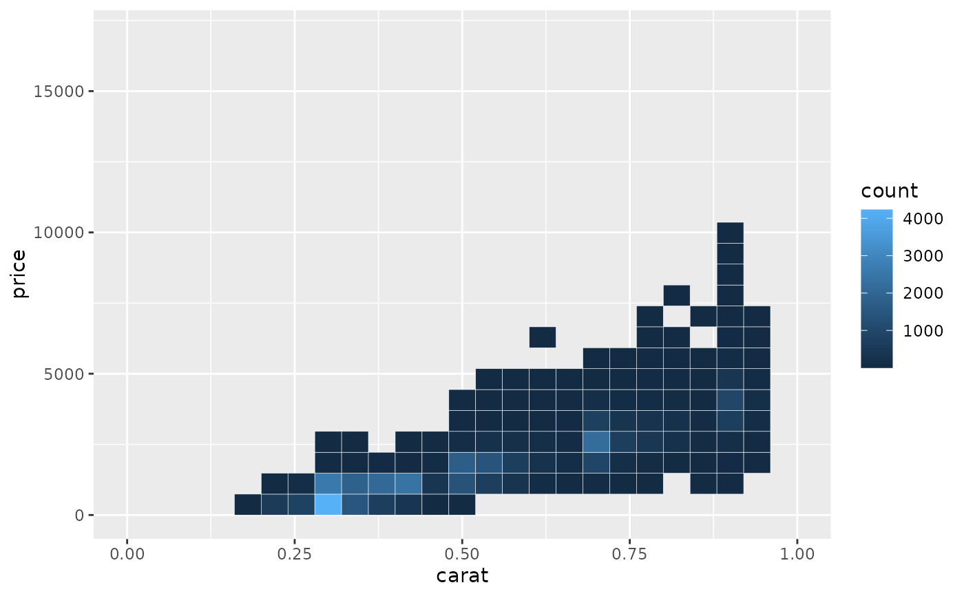
# When zooming the coordinate system, we see a subset of original 50 bins,
# displayed bigger
d + coord_cartesian(xlim = c(0, 1))