ggplot2 can not draw true 3D surfaces, but you can use geom_contour(),
geom_contour_filled(), and geom_tile() to visualise 3D surfaces in 2D.
These functions require regular data, where the x and y coordinates
form an equally spaced grid, and each combination of x and y appears
once. Missing values of z are allowed, but contouring will only work for
grid points where all four corners are non-missing. If you have irregular
data, you'll need to first interpolate on to a grid before visualising,
using interp::interp(), akima::bilinear(), or similar.
Usage
geom_contour(
  mapping = NULL,
  data = NULL,
  stat = "contour",
  position = "identity",
  ...,
  bins = NULL,
  binwidth = NULL,
  breaks = NULL,
  arrow = NULL,
  arrow.fill = NULL,
  lineend = "butt",
  linejoin = "round",
  linemitre = 10,
  na.rm = FALSE,
  show.legend = NA,
  inherit.aes = TRUE
)

geom_contour_filled(
  mapping = NULL,
  data = NULL,
  stat = "contour_filled",
  position = "identity",
  ...,
  bins = NULL,
  binwidth = NULL,
  breaks = NULL,
  rule = "evenodd",
  lineend = "butt",
  linejoin = "round",
  linemitre = 10,
  na.rm = FALSE,
  show.legend = NA,
  inherit.aes = TRUE
)

stat_contour(
  mapping = NULL,
  data = NULL,
  geom = "contour",
  position = "identity",
  ...,
  bins = NULL,
  binwidth = NULL,
  breaks = NULL,
  na.rm = FALSE,
  show.legend = NA,
  inherit.aes = TRUE
)

stat_contour_filled(
  mapping = NULL,
  data = NULL,
  geom = "contour_filled",
  position = "identity",
  ...,
  bins = NULL,
  binwidth = NULL,
  breaks = NULL,
  na.rm = FALSE,
  show.legend = NA,
  inherit.aes = TRUE
)
Arguments
- mapping
Set of aesthetic mappings created by
aes(). If specified andinherit.aes = TRUE(the default), it is combined with the default mapping at the top level of the plot. You must supplymappingif there is no plot mapping.- data
The data to be displayed in this layer. There are three options:
NULL(default): the data is inherited from the plot data as specified in the call toggplot().A
data.frame, or other object, will override the plot data. All objects will be fortified to produce a data frame. Seefortify()for which variables will be created.A
functionwill be called with a single argument, the plot data. The return value must be adata.frame, and will be used as the layer data. Afunctioncan be created from aformula(e.g.~ head(.x, 10)).
- stat
The statistical transformation to use on the data for this layer. When using a
geom_*()function to construct a layer, thestatargument can be used to override the default coupling between geoms and stats. Thestatargument accepts the following:A
Statggproto subclass, for exampleStatCount.A string naming the stat. To give the stat as a string, strip the function name of the
stat_prefix. For example, to usestat_count(), give the stat as"count".For more information and other ways to specify the stat, see the layer stat documentation.
- position
A position adjustment to use on the data for this layer. This can be used in various ways, including to prevent overplotting and improving the display. The
positionargument accepts the following:The result of calling a position function, such as
position_jitter(). This method allows for passing extra arguments to the position.A string naming the position adjustment. To give the position as a string, strip the function name of the
position_prefix. For example, to useposition_jitter(), give the position as"jitter".For more information and other ways to specify the position, see the layer position documentation.
- ...
Other arguments passed on to
layer()'sparamsargument. These arguments broadly fall into one of 4 categories below. Notably, further arguments to thepositionargument, or aesthetics that are required can not be passed through.... Unknown arguments that are not part of the 4 categories below are ignored.Static aesthetics that are not mapped to a scale, but are at a fixed value and apply to the layer as a whole. For example,
colour = "red"orlinewidth = 3. The geom's documentation has an Aesthetics section that lists the available options. The 'required' aesthetics cannot be passed on to theparams. Please note that while passing unmapped aesthetics as vectors is technically possible, the order and required length is not guaranteed to be parallel to the input data.When constructing a layer using a
stat_*()function, the...argument can be used to pass on parameters to thegeompart of the layer. An example of this isstat_density(geom = "area", outline.type = "both"). The geom's documentation lists which parameters it can accept.Inversely, when constructing a layer using a
geom_*()function, the...argument can be used to pass on parameters to thestatpart of the layer. An example of this isgeom_area(stat = "density", adjust = 0.5). The stat's documentation lists which parameters it can accept.The
key_glyphargument oflayer()may also be passed on through.... This can be one of the functions described as key glyphs, to change the display of the layer in the legend.
- bins
Number of contour bins. Overridden by
breaks.- binwidth
The width of the contour bins. Overridden by
bins.- breaks
One of:
Numeric vector to set the contour breaks
A function that takes the range of the data and binwidth as input and returns breaks as output. A function can be created from a formula (e.g. ~ fullseq(.x, .y)).
Overrides
binwidthandbins. By default, this is a vector of length ten withpretty()breaks.- arrow
Arrow specification. Can be created by
grid::arrow()orNULLto not draw an arrow.- arrow.fill
Fill colour to use for closed arrowheads.
NULLmeans usecolouraesthetic.- lineend
Line end style, one of
"round","butt"or"square".- linejoin
Line join style, one of
"round","mitre"or"bevel".- linemitre
Line mitre limit, a number greater than 1.
- na.rm
If
FALSE, the default, missing values are removed with a warning. IfTRUE, missing values are silently removed.- show.legend
Logical. Should this layer be included in the legends?
NA, the default, includes if any aesthetics are mapped.FALSEnever includes, andTRUEalways includes. It can also be a named logical vector to finely select the aesthetics to display. To include legend keys for all levels, even when no data exists, useTRUE. IfNA, all levels are shown in legend, but unobserved levels are omitted.- inherit.aes
If
FALSE, overrides the default aesthetics, rather than combining with them. This is most useful for helper functions that define both data and aesthetics and shouldn't inherit behaviour from the default plot specification, e.g.annotation_borders().- rule
Either
"evenodd"or"winding". If polygons with holes are being drawn (using thesubgroupaesthetic) this argument defines how the hole coordinates are interpreted. See the examples ingrid::pathGrob()for an explanation.- geom
The geometric object to use to display the data for this layer. When using a
stat_*()function to construct a layer, thegeomargument can be used to override the default coupling between stats and geoms. Thegeomargument accepts the following:A
Geomggproto subclass, for exampleGeomPoint.A string naming the geom. To give the geom as a string, strip the function name of the
geom_prefix. For example, to usegeom_point(), give the geom as"point".For more information and other ways to specify the geom, see the layer geom documentation.
Computed variables
These are calculated by the 'stat' part of layers and can be accessed with delayed evaluation. The computed variables differ somewhat for contour lines (computed by stat_contour()) and contour bands (filled contours, computed by stat_contour_filled()). The variables nlevel and piece are available for both, whereas level_low, level_high, and level_mid are only available for bands. The variable level is a numeric or a factor depending on whether lines or bands are calculated.
after_stat(level)
Height of contour. For contour lines, this is a numeric vector that represents bin boundaries. For contour bands, this is an ordered factor that represents bin ranges.after_stat(level_low),after_stat(level_high),after_stat(level_mid)
(contour bands only) Lower and upper bin boundaries for each band, as well as the mid point between boundaries.after_stat(nlevel)
Height of contour, scaled to a maximum of 1.after_stat(piece)
Contour piece (an integer).
Dropped variables
zAfter contouring, the z values of individual data points are no longer available.
See also
geom_density_2d(): 2d density contours
Aesthetics
geom_contour() understands the following aesthetics. Required aesthetics are displayed in bold and defaults are displayed for optional aesthetics:
| • | x | |
| • | y | |
| • | alpha | → NA |
| • | colour | → via theme() |
| • | group | → inferred |
| • | linetype | → via theme() |
| • | linewidth | → via theme() |
| • | weight | → 1 |
geom_contour_filled() understands the following aesthetics. Required aesthetics are displayed in bold and defaults are displayed for optional aesthetics:
| • | x | |
| • | y | |
| • | alpha | → NA |
| • | colour | → via theme() |
| • | fill | → via theme() |
| • | group | → inferred |
| • | linetype | → via theme() |
| • | linewidth | → via theme() |
| • | subgroup | → NULL |
stat_contour() understands the following aesthetics. Required aesthetics are displayed in bold and defaults are displayed for optional aesthetics:
| • | x | |
| • | y | |
| • | z | |
| • | group | → inferred |
| • | order | → after_stat(level) |
stat_contour_filled() understands the following aesthetics. Required aesthetics are displayed in bold and defaults are displayed for optional aesthetics:
| • | x | |
| • | y | |
| • | z | |
| • | fill | → after_stat(level) |
| • | group | → inferred |
| • | order | → after_stat(level) |
Learn more about setting these aesthetics in vignette("ggplot2-specs").
Examples
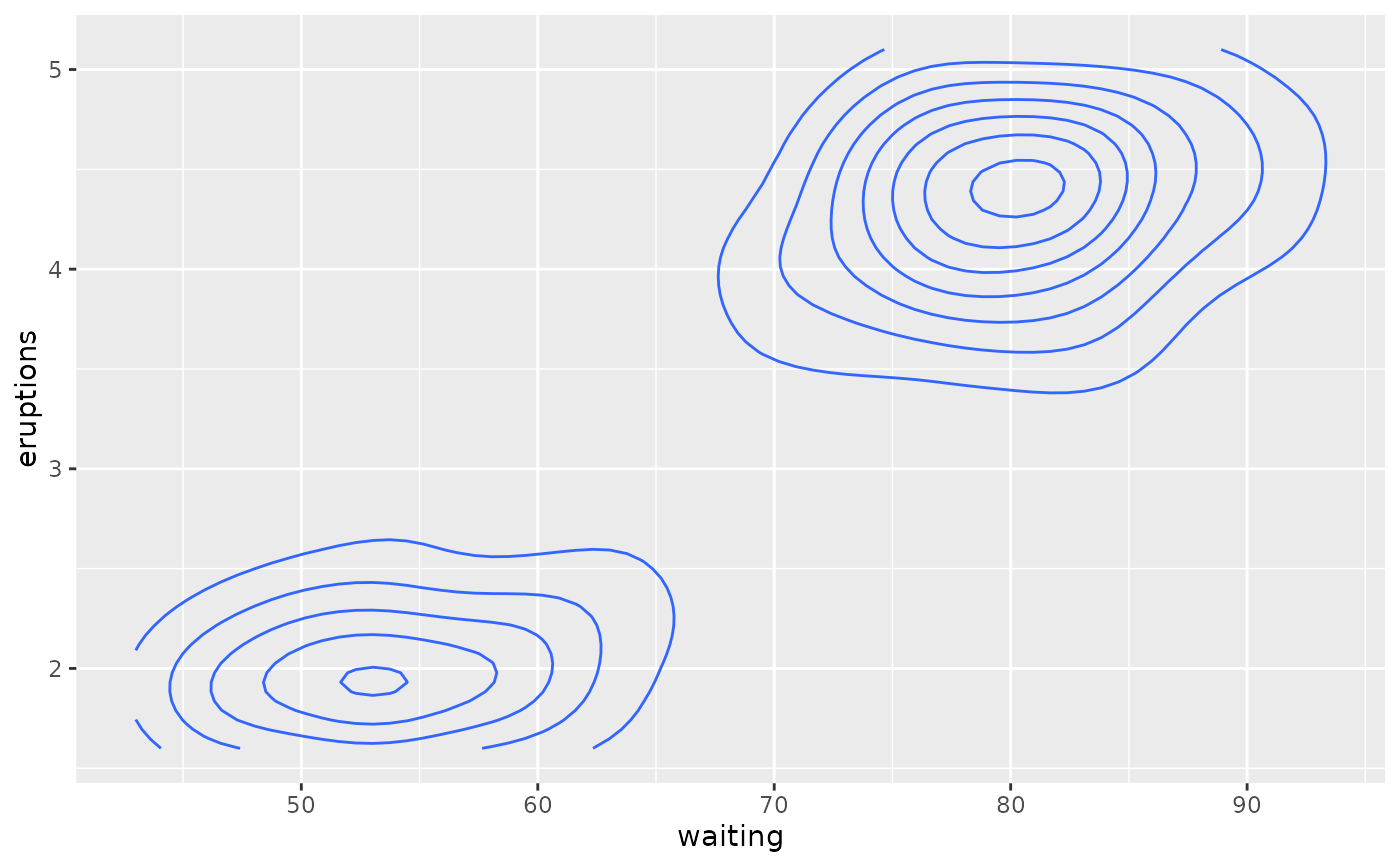
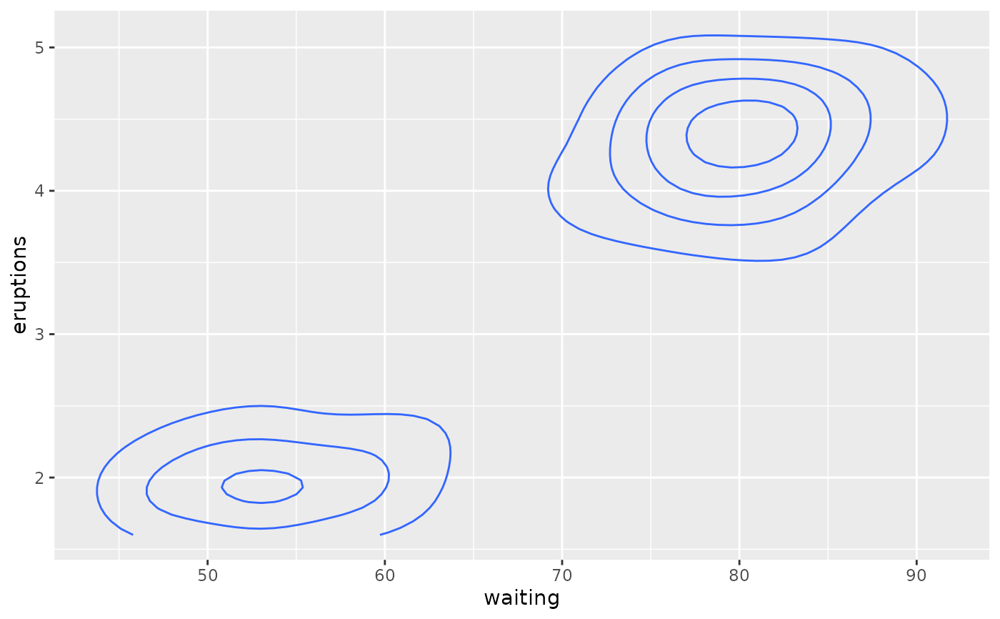
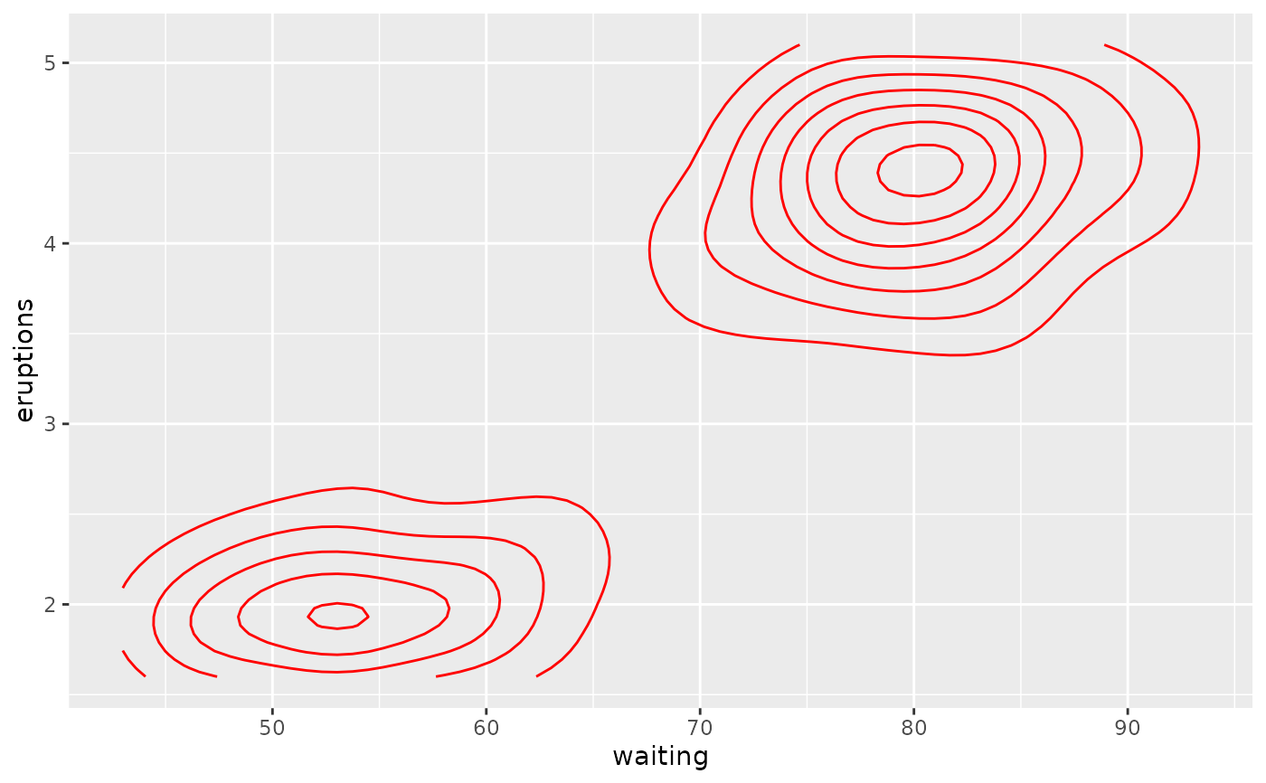
# Basic plot
v <- ggplot(faithfuld, aes(waiting, eruptions, z = density))
v + geom_contour()
 # Or compute from raw data
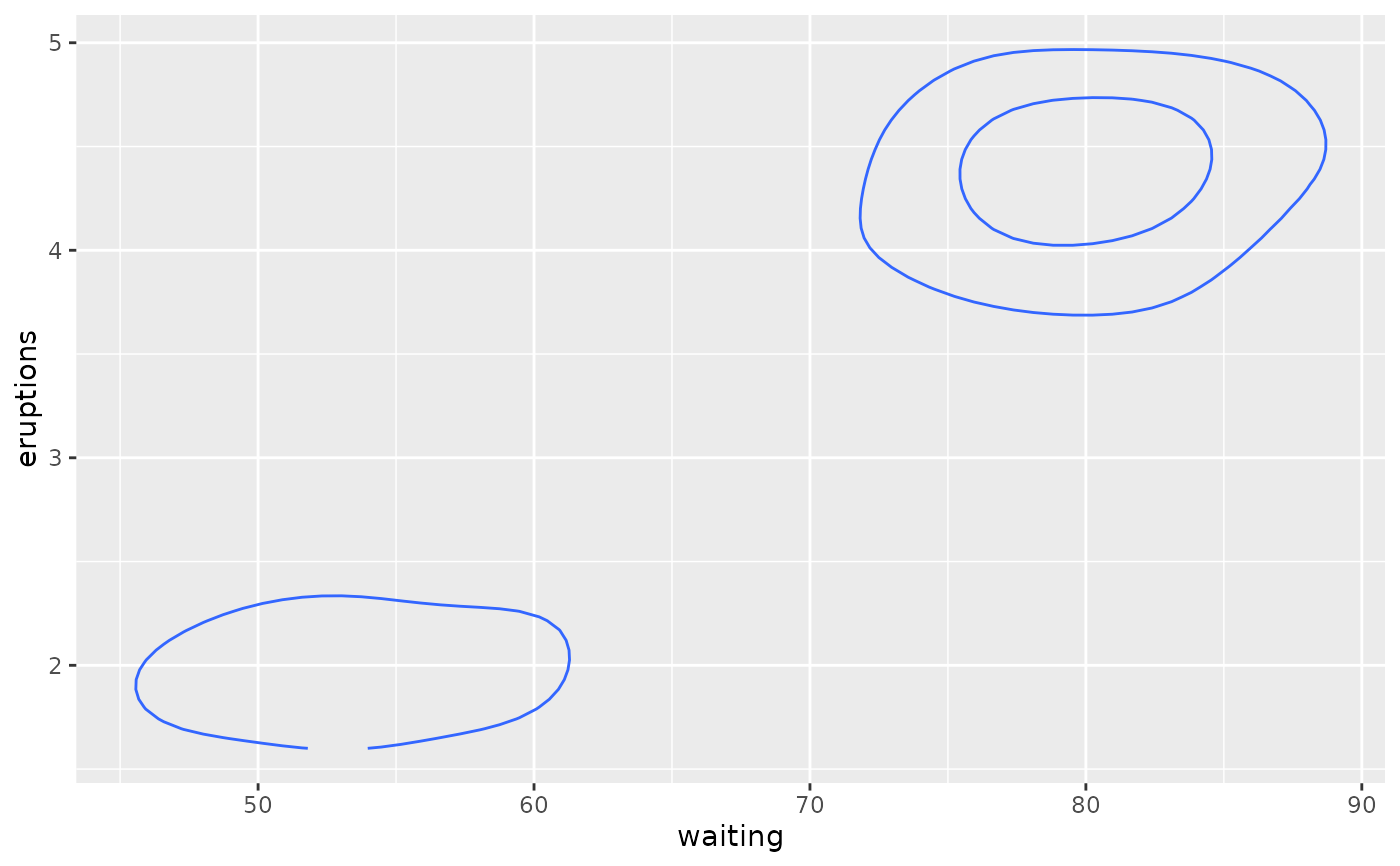
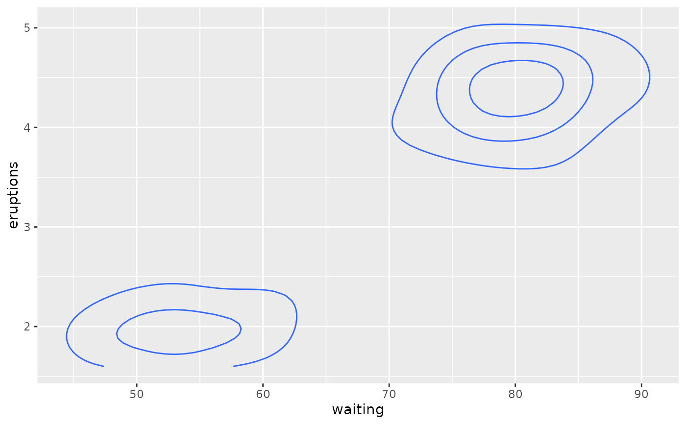
ggplot(faithful, aes(waiting, eruptions)) +
geom_density_2d()
# Or compute from raw data
ggplot(faithful, aes(waiting, eruptions)) +
geom_density_2d()
 # \donttest{
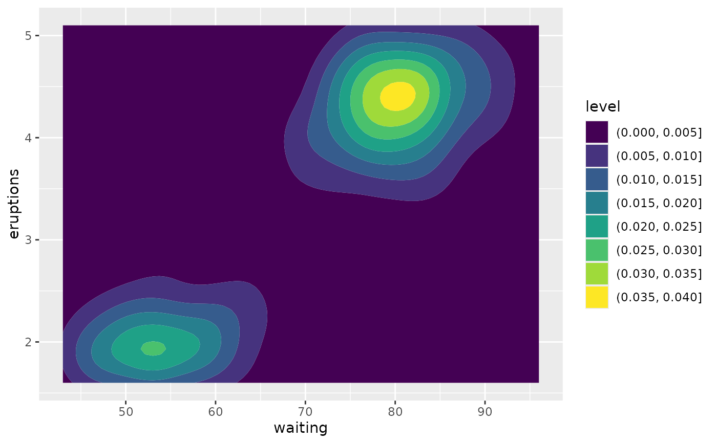
# use geom_contour_filled() for filled contours
v + geom_contour_filled()
# \donttest{
# use geom_contour_filled() for filled contours
v + geom_contour_filled()
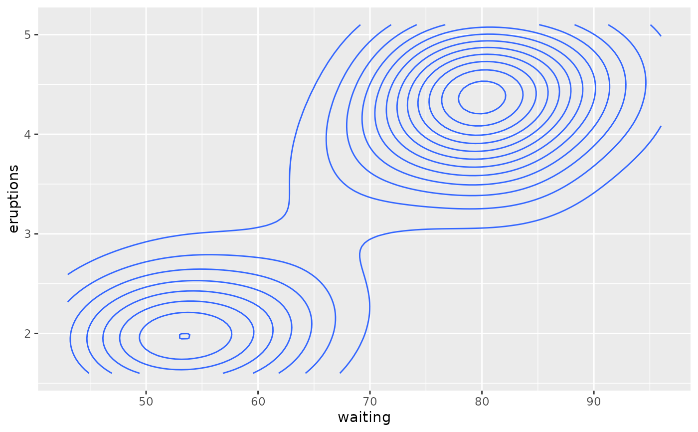
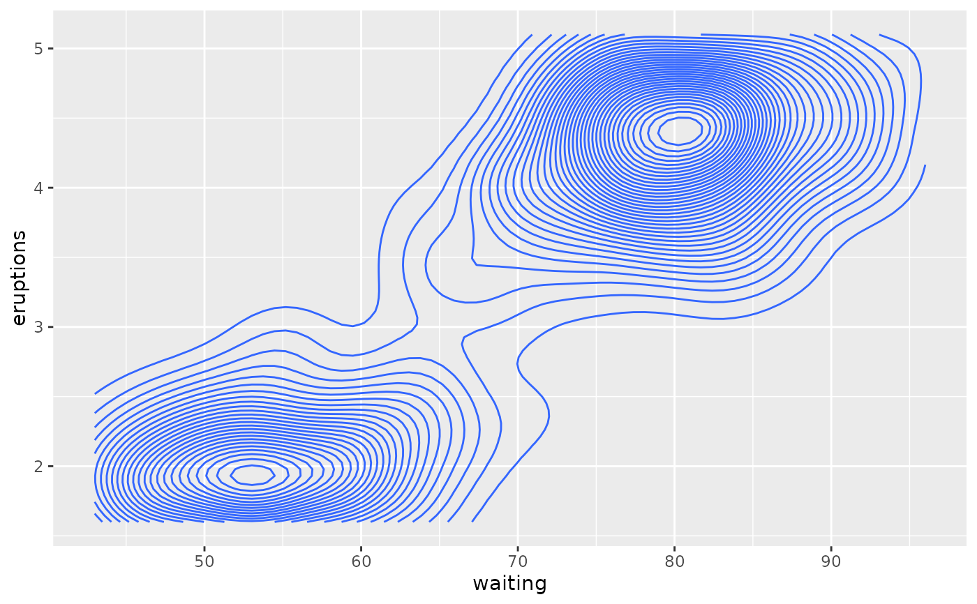
 # Setting bins creates evenly spaced contours in the range of the data
v + geom_contour(bins = 3)
# Setting bins creates evenly spaced contours in the range of the data
v + geom_contour(bins = 3)
 v + geom_contour(bins = 5)
 # Setting binwidth does the same thing, parameterised by the distance
# between contours
v + geom_contour(binwidth = 0.01)
# Setting binwidth does the same thing, parameterised by the distance
# between contours
v + geom_contour(binwidth = 0.01)
 v + geom_contour(binwidth = 0.001)
 # Other parameters
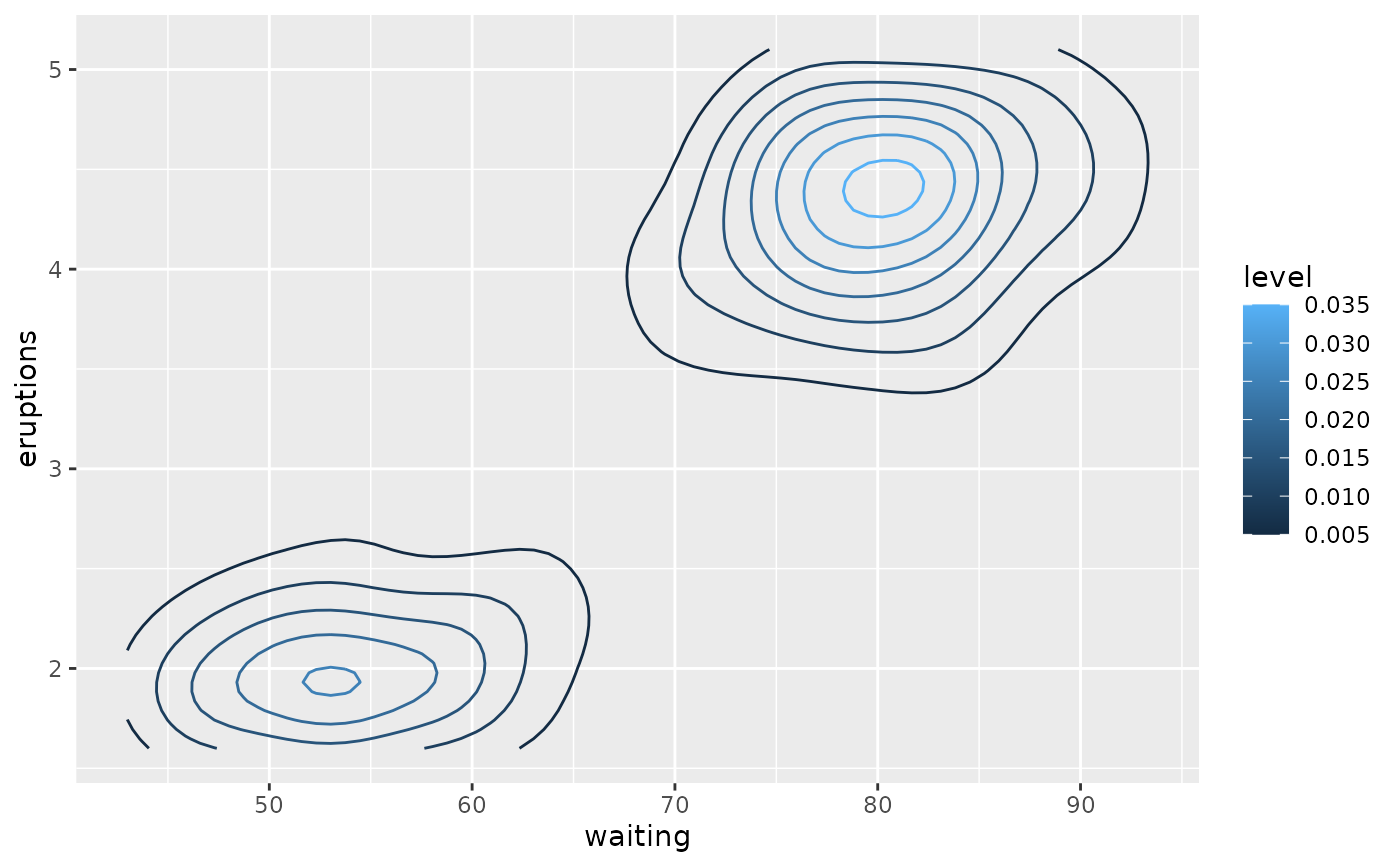
v + geom_contour(aes(colour = after_stat(level)))
# Other parameters
v + geom_contour(aes(colour = after_stat(level)))
 v + geom_contour(colour = "red")
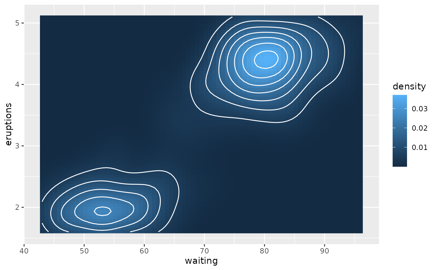
 v + geom_raster(aes(fill = density)) +
geom_contour(colour = "white")
v + geom_raster(aes(fill = density)) +
geom_contour(colour = "white")
 # }
# }