Summarise y values at unique/binned x
Source:R/stat-summary-bin.R, R/stat-summary.R
stat_summary.Rdstat_summary() operates on unique x or y; stat_summary_bin()
operates on binned x or y. They are more flexible versions of
stat_bin(): instead of just counting, they can compute any
aggregate.
Usage
stat_summary_bin(
  mapping = NULL,
  data = NULL,
  geom = "pointrange",
  position = "identity",
  ...,
  fun.data = NULL,
  fun = NULL,
  fun.max = NULL,
  fun.min = NULL,
  fun.args = list(),
  bins = 30,
  binwidth = NULL,
  breaks = NULL,
  na.rm = FALSE,
  orientation = NA,
  show.legend = NA,
  inherit.aes = TRUE,
  fun.y = deprecated(),
  fun.ymin = deprecated(),
  fun.ymax = deprecated()
)

stat_summary(
  mapping = NULL,
  data = NULL,
  geom = "pointrange",
  position = "identity",
  ...,
  fun.data = NULL,
  fun = NULL,
  fun.max = NULL,
  fun.min = NULL,
  fun.args = list(),
  na.rm = FALSE,
  orientation = NA,
  show.legend = NA,
  inherit.aes = TRUE,
  fun.y = deprecated(),
  fun.ymin = deprecated(),
  fun.ymax = deprecated()
)
Arguments
- mapping
Set of aesthetic mappings created by
aes(). If specified andinherit.aes = TRUE(the default), it is combined with the default mapping at the top level of the plot. You must supplymappingif there is no plot mapping.- data
The data to be displayed in this layer. There are three options:
If
NULL, the default, the data is inherited from the plot data as specified in the call toggplot().A
data.frame, or other object, will override the plot data. All objects will be fortified to produce a data frame. Seefortify()for which variables will be created.A
functionwill be called with a single argument, the plot data. The return value must be adata.frame, and will be used as the layer data. Afunctioncan be created from aformula(e.g.~ head(.x, 10)).- geom
The geometric object to use to display the data for this layer. When using a
stat_*()function to construct a layer, thegeomargument can be used to override the default coupling between stats and geoms. Thegeomargument accepts the following:A
Geomggproto subclass, for exampleGeomPoint.A string naming the geom. To give the geom as a string, strip the function name of the
geom_prefix. For example, to usegeom_point(), give the geom as"point".For more information and other ways to specify the geom, see the layer geom documentation.
- position
A position adjustment to use on the data for this layer. This can be used in various ways, including to prevent overplotting and improving the display. The
positionargument accepts the following:The result of calling a position function, such as
position_jitter(). This method allows for passing extra arguments to the position.A string naming the position adjustment. To give the position as a string, strip the function name of the
position_prefix. For example, to useposition_jitter(), give the position as"jitter".For more information and other ways to specify the position, see the layer position documentation.
- ...
Other arguments passed on to
layer()'sparamsargument. These arguments broadly fall into one of 4 categories below. Notably, further arguments to thepositionargument, or aesthetics that are required can not be passed through.... Unknown arguments that are not part of the 4 categories below are ignored.Static aesthetics that are not mapped to a scale, but are at a fixed value and apply to the layer as a whole. For example,
colour = "red"orlinewidth = 3. The geom's documentation has an Aesthetics section that lists the available options. The 'required' aesthetics cannot be passed on to theparams. Please note that while passing unmapped aesthetics as vectors is technically possible, the order and required length is not guaranteed to be parallel to the input data.When constructing a layer using a
stat_*()function, the...argument can be used to pass on parameters to thegeompart of the layer. An example of this isstat_density(geom = "area", outline.type = "both"). The geom's documentation lists which parameters it can accept.Inversely, when constructing a layer using a
geom_*()function, the...argument can be used to pass on parameters to thestatpart of the layer. An example of this isgeom_area(stat = "density", adjust = 0.5). The stat's documentation lists which parameters it can accept.The
key_glyphargument oflayer()may also be passed on through.... This can be one of the functions described as key glyphs, to change the display of the layer in the legend.
- fun.data
A function that is given the complete data and should return a data frame with variables
ymin,y, andymax.- fun.min, fun, fun.max
Alternatively, supply three individual functions that are each passed a vector of values and should return a single number.
- fun.args
Optional additional arguments passed on to the functions.
- bins
Number of bins. Overridden by
binwidth. Defaults to 30.- binwidth
The width of the bins. Can be specified as a numeric value or as a function that takes x after scale transformation as input and returns a single numeric value. When specifying a function along with a grouping structure, the function will be called once per group. The default is to use the number of bins in
bins, covering the range of the data. You should always override this value, exploring multiple widths to find the best to illustrate the stories in your data.The bin width of a date variable is the number of days in each time; the bin width of a time variable is the number of seconds.
- breaks
Alternatively, you can supply a numeric vector giving the bin boundaries. Overrides
binwidthandbins.- na.rm
If
FALSE, the default, missing values are removed with a warning. IfTRUE, missing values are silently removed.- orientation
The orientation of the layer. The default (
NA) automatically determines the orientation from the aesthetic mapping. In the rare event that this fails it can be given explicitly by settingorientationto either"x"or"y". See the Orientation section for more detail.- show.legend
logical. Should this layer be included in the legends?
NA, the default, includes if any aesthetics are mapped.FALSEnever includes, andTRUEalways includes. It can also be a named logical vector to finely select the aesthetics to display. To include legend keys for all levels, even when no data exists, useTRUE. IfNA, all levels are shown in legend, but unobserved levels are omitted.- inherit.aes
If
FALSE, overrides the default aesthetics, rather than combining with them. This is most useful for helper functions that define both data and aesthetics and shouldn't inherit behaviour from the default plot specification, e.g.annotation_borders().- fun.ymin, fun.y, fun.ymax
![[Deprecated]](figures/lifecycle-deprecated.svg) Use the
versions specified above instead.
Use the
versions specified above instead.
Orientation
This geom treats each axis differently and, thus, can thus have two orientations. Often the orientation is easy to deduce from a combination of the given mappings and the types of positional scales in use. Thus, ggplot2 will by default try to guess which orientation the layer should have. Under rare circumstances, the orientation is ambiguous and guessing may fail. In that case the orientation can be specified directly using the orientation parameter, which can be either "x" or "y". The value gives the axis that the geom should run along, "x" being the default orientation you would expect for the geom.
Summary functions
You can either supply summary functions individually (fun,
fun.max, fun.min), or as a single function (fun.data):
- fun.data
Complete summary function. Should take numeric vector as input and return data frame as output
- fun.min
min summary function (should take numeric vector and return single number)
- fun
main summary function (should take numeric vector and return single number)
- fun.max
max summary function (should take numeric vector and return single number)
A simple vector function is easiest to work with as you can return a single
number, but is somewhat less flexible. If your summary function computes
multiple values at once (e.g. min and max), use fun.data.
fun.data will receive data as if it was oriented along the x-axis and
should return a data.frame that corresponds to that orientation. The layer
will take care of flipping the input and output if it is oriented along the
y-axis.
If no aggregation functions are supplied, will default to
mean_se().
See also
geom_errorbar(), geom_pointrange(),
geom_linerange(), geom_crossbar() for geoms to
display summarised data
Aesthetics
stat_summary() understands the following aesthetics. Required aesthetics are displayed in bold and defaults are displayed for optional aesthetics:
| • | x | |
| • | y | |
| • | group | → inferred |
Learn more about setting these aesthetics in vignette("ggplot2-specs").
Examples
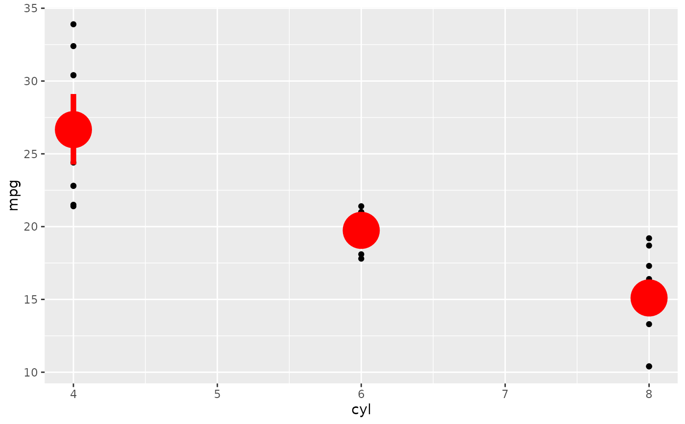
d <- ggplot(mtcars, aes(cyl, mpg)) + geom_point()
d + stat_summary(fun.data = "mean_cl_boot", colour = "red", linewidth = 2, size = 3)
 # Orientation follows the discrete axis
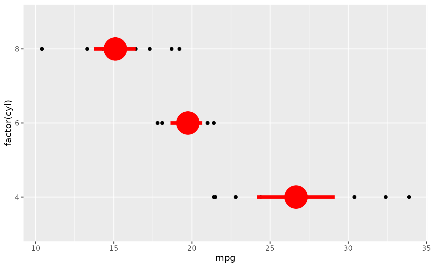
ggplot(mtcars, aes(mpg, factor(cyl))) +
geom_point() +
stat_summary(fun.data = "mean_cl_boot", colour = "red", linewidth = 2, size = 3)
# Orientation follows the discrete axis
ggplot(mtcars, aes(mpg, factor(cyl))) +
geom_point() +
stat_summary(fun.data = "mean_cl_boot", colour = "red", linewidth = 2, size = 3)
 # You can supply individual functions to summarise the value at
# each x:
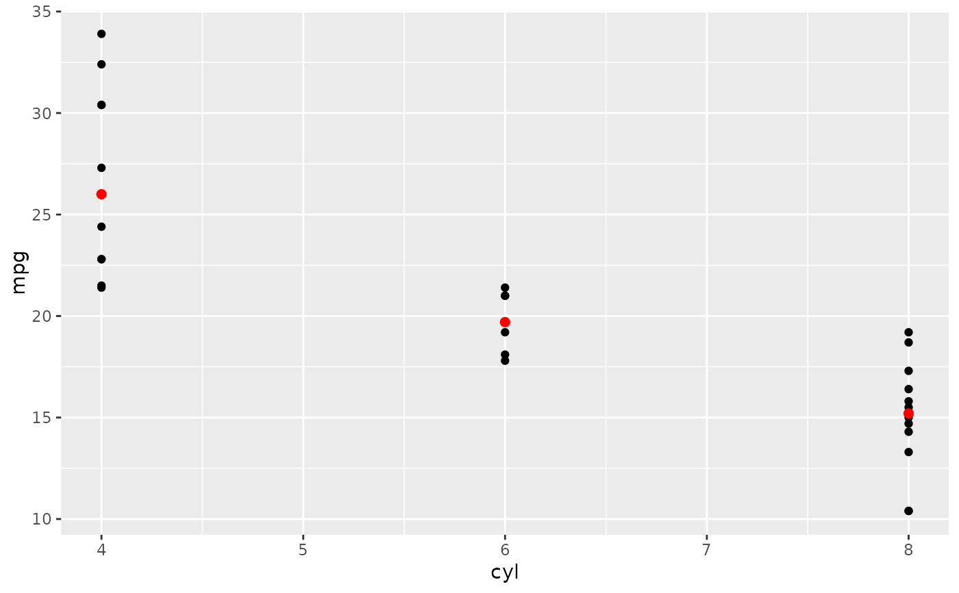
d + stat_summary(fun = "median", colour = "red", size = 2, geom = "point")
# You can supply individual functions to summarise the value at
# each x:
d + stat_summary(fun = "median", colour = "red", size = 2, geom = "point")
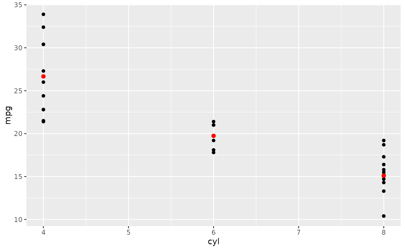
 d + stat_summary(fun = "mean", colour = "red", size = 2, geom = "point")
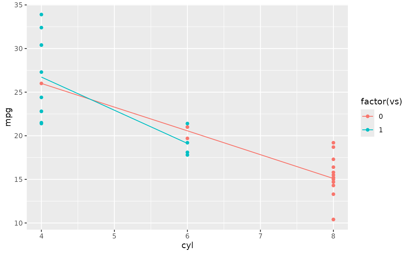
 d + aes(colour = factor(vs)) + stat_summary(fun = mean, geom="line")
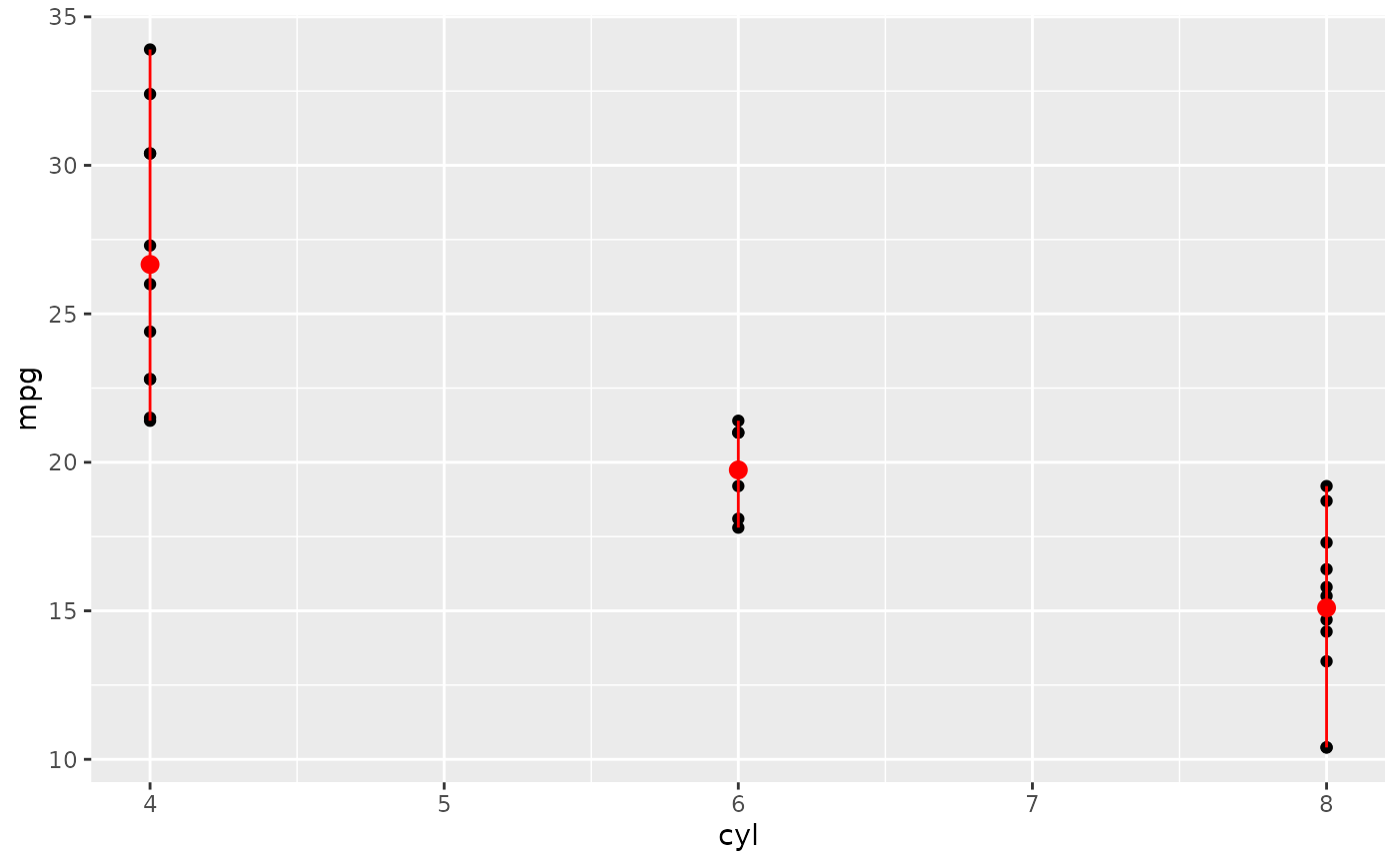
 d + stat_summary(fun = mean, fun.min = min, fun.max = max, colour = "red")
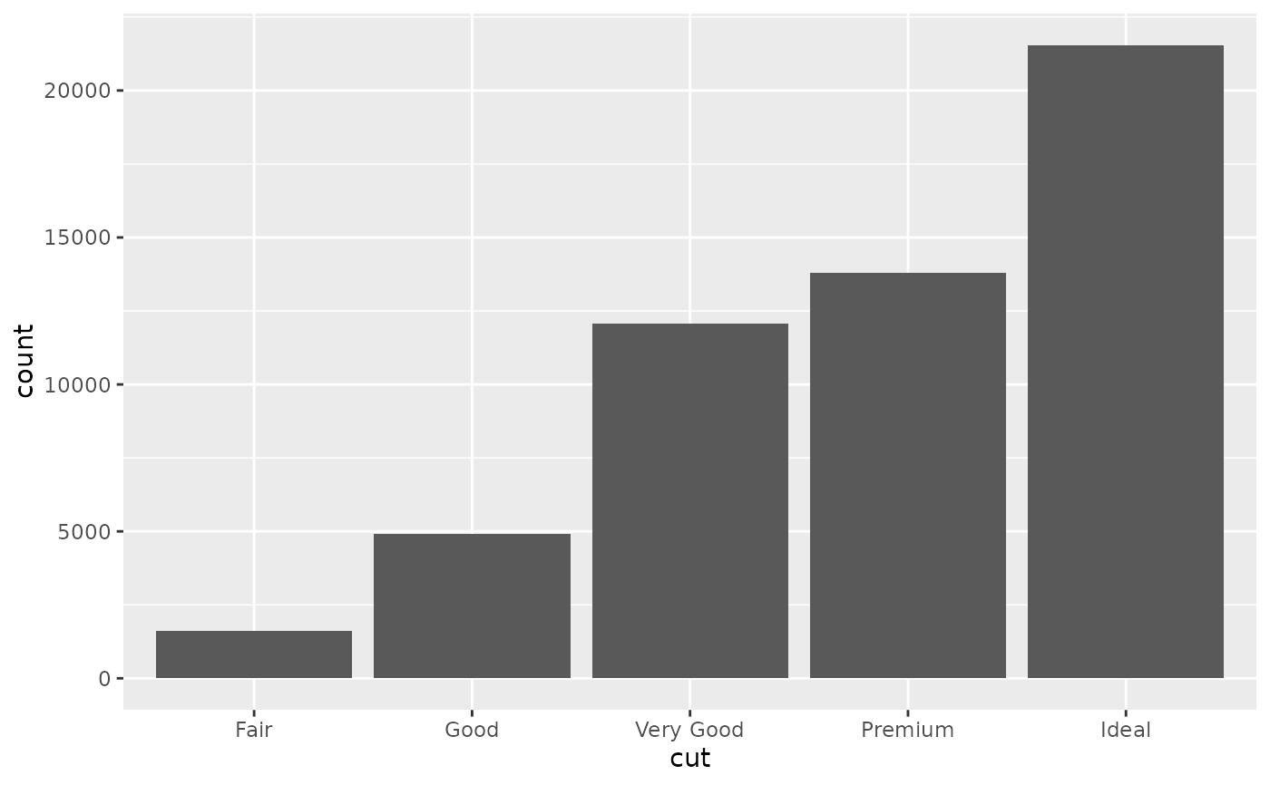
 d <- ggplot(diamonds, aes(cut))
d + geom_bar()
d <- ggplot(diamonds, aes(cut))
d + geom_bar()
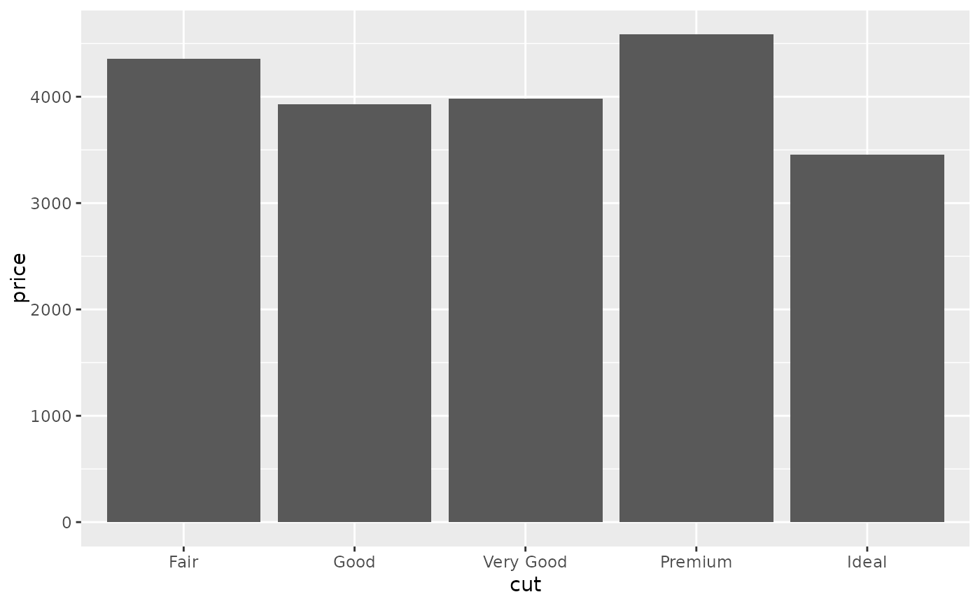
 d + stat_summary(aes(y = price), fun = "mean", geom = "bar")
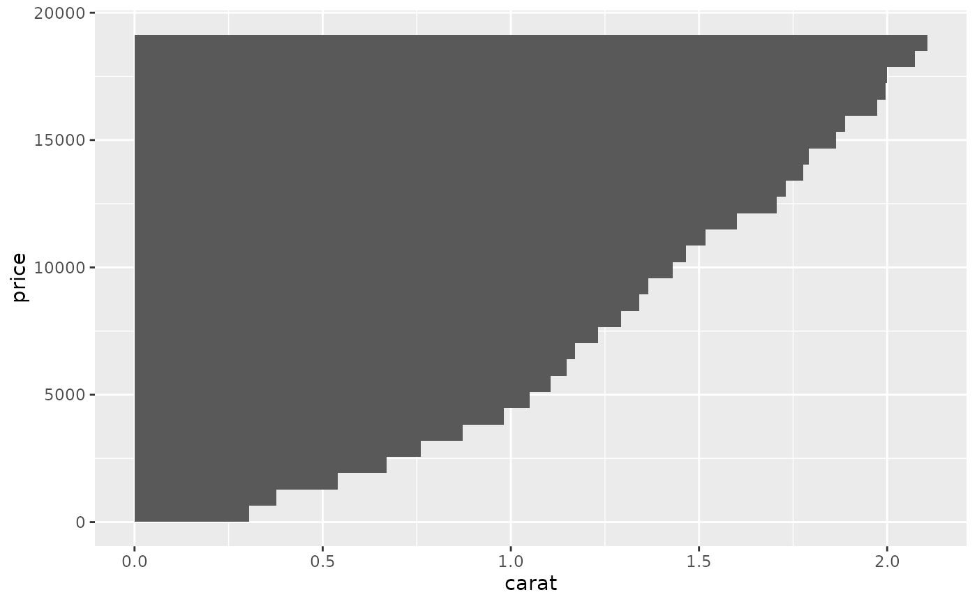
 # Orientation of stat_summary_bin is ambiguous and must be specified directly
ggplot(diamonds, aes(carat, price)) +
stat_summary_bin(fun = "mean", geom = "bar", orientation = 'y')
# Orientation of stat_summary_bin is ambiguous and must be specified directly
ggplot(diamonds, aes(carat, price)) +
stat_summary_bin(fun = "mean", geom = "bar", orientation = 'y')
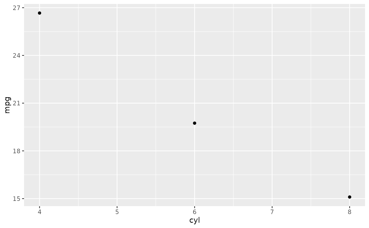
 # \donttest{
# Don't use ylim to zoom into a summary plot - this throws the
# data away
p <- ggplot(mtcars, aes(cyl, mpg)) +
stat_summary(fun = "mean", geom = "point")
p
# \donttest{
# Don't use ylim to zoom into a summary plot - this throws the
# data away
p <- ggplot(mtcars, aes(cyl, mpg)) +
stat_summary(fun = "mean", geom = "point")
p
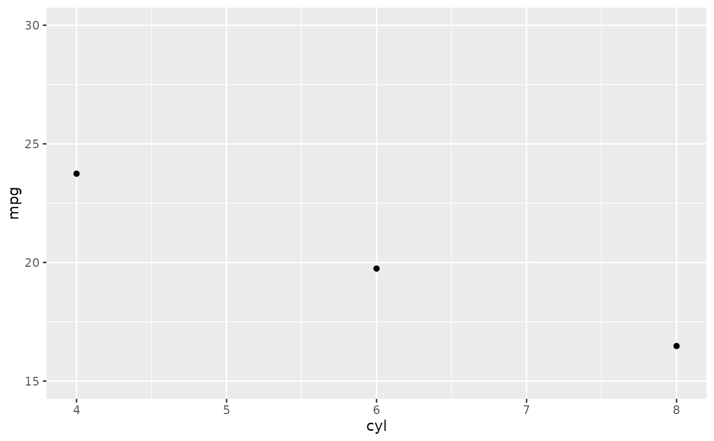
 p + ylim(15, 30)
#> Warning: Removed 9 rows containing non-finite outside the scale range
#> (`stat_summary()`).
p + ylim(15, 30)
#> Warning: Removed 9 rows containing non-finite outside the scale range
#> (`stat_summary()`).
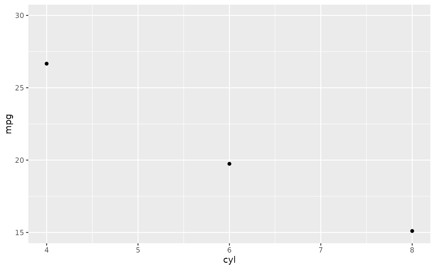
 # Instead use coord_cartesian
p + coord_cartesian(ylim = c(15, 30))
# Instead use coord_cartesian
p + coord_cartesian(ylim = c(15, 30))
 # A set of useful summary functions is provided from the Hmisc package:
stat_sum_df <- function(fun, geom="crossbar", ...) {
stat_summary(fun.data = fun, colour = "red", geom = geom, width = 0.2, ...)
}
d <- ggplot(mtcars, aes(cyl, mpg)) + geom_point()
# The crossbar geom needs grouping to be specified when used with
# a continuous x axis.
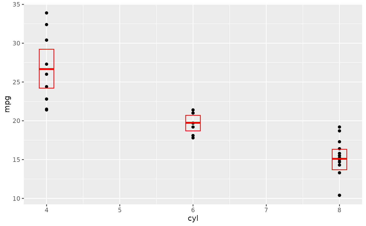
d + stat_sum_df("mean_cl_boot", mapping = aes(group = cyl))
# A set of useful summary functions is provided from the Hmisc package:
stat_sum_df <- function(fun, geom="crossbar", ...) {
stat_summary(fun.data = fun, colour = "red", geom = geom, width = 0.2, ...)
}
d <- ggplot(mtcars, aes(cyl, mpg)) + geom_point()
# The crossbar geom needs grouping to be specified when used with
# a continuous x axis.
d + stat_sum_df("mean_cl_boot", mapping = aes(group = cyl))
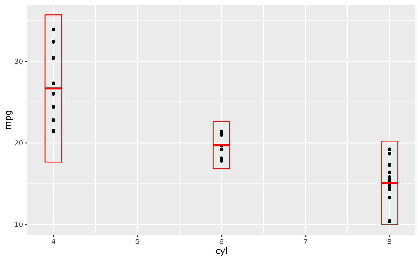
 d + stat_sum_df("mean_sdl", mapping = aes(group = cyl))
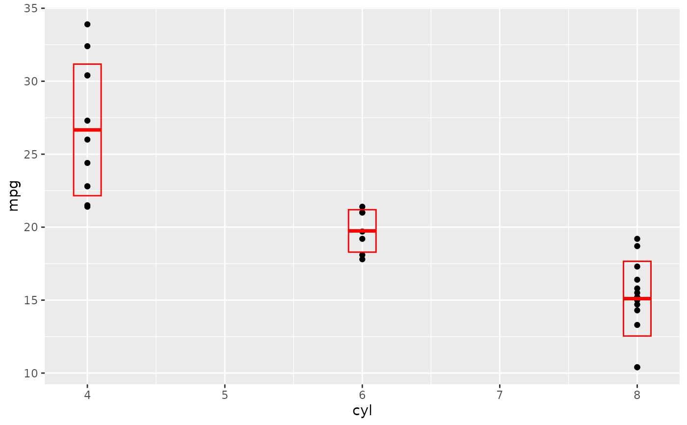
 d + stat_sum_df("mean_sdl", fun.args = list(mult = 1), mapping = aes(group = cyl))
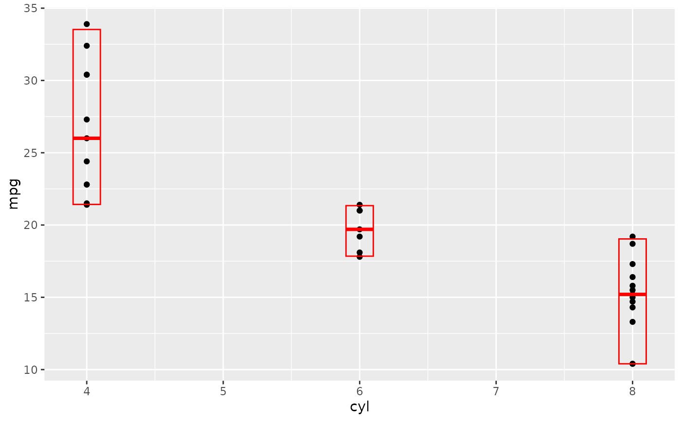
 d + stat_sum_df("median_hilow", mapping = aes(group = cyl))
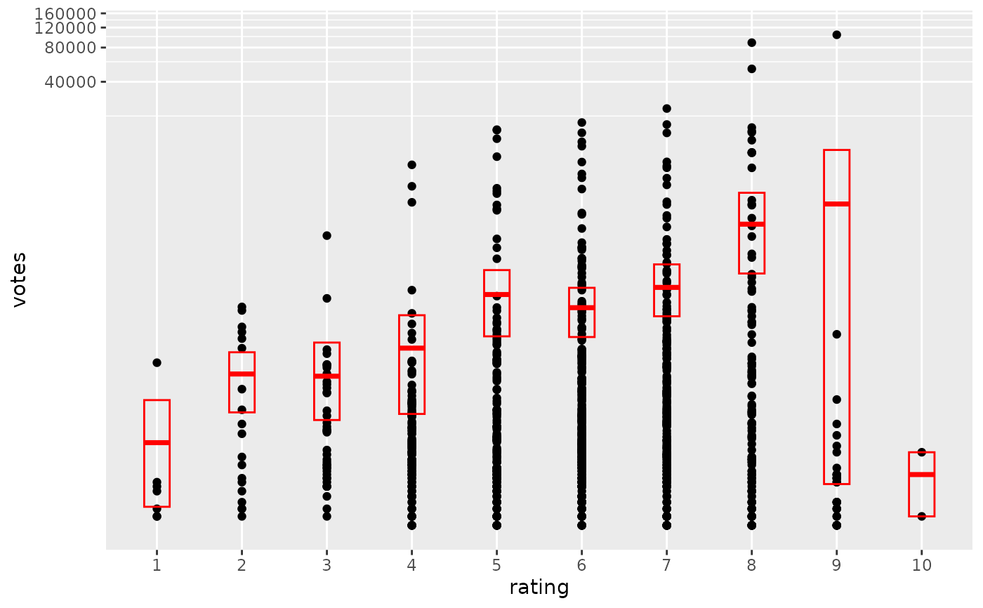
 # An example with highly skewed distributions:
if (require("ggplot2movies")) {
set.seed(596)
mov <- movies[sample(nrow(movies), 1000), ]
m2 <-
ggplot(mov, aes(x = factor(round(rating)), y = votes)) +
geom_point()
m2 <-
m2 +
stat_summary(
fun.data = "mean_cl_boot",
geom = "crossbar",
colour = "red", width = 0.3
) +
xlab("rating")
m2
# Notice how the overplotting skews off visual perception of the mean
# supplementing the raw data with summary statistics is _very_ important
# Next, we'll look at votes on a log scale.
# Transforming the scale means the data are transformed
# first, after which statistics are computed:
m2 + scale_y_log10()
# Transforming the coordinate system occurs after the
# statistic has been computed. This means we're calculating the summary on the raw data
# and stretching the geoms onto the log scale. Compare the widths of the
# standard errors.
m2 + coord_transform(y="log10")
}
# An example with highly skewed distributions:
if (require("ggplot2movies")) {
set.seed(596)
mov <- movies[sample(nrow(movies), 1000), ]
m2 <-
ggplot(mov, aes(x = factor(round(rating)), y = votes)) +
geom_point()
m2 <-
m2 +
stat_summary(
fun.data = "mean_cl_boot",
geom = "crossbar",
colour = "red", width = 0.3
) +
xlab("rating")
m2
# Notice how the overplotting skews off visual perception of the mean
# supplementing the raw data with summary statistics is _very_ important
# Next, we'll look at votes on a log scale.
# Transforming the scale means the data are transformed
# first, after which statistics are computed:
m2 + scale_y_log10()
# Transforming the coordinate system occurs after the
# statistic has been computed. This means we're calculating the summary on the raw data
# and stretching the geoms onto the log scale. Compare the widths of the
# standard errors.
m2 + coord_transform(y="log10")
}
 # }
# }