Reference lines: horizontal, vertical, and diagonal

These geoms add reference lines (sometimes called rules) to a plot, either horizontal, vertical, or diagonal (specified by slope and intercept). These are useful for annotating plots.

Usage

geom_abline(
  mapping = NULL,
  data = NULL,
  ...,
  slope,
  intercept,
  na.rm = FALSE,
  show.legend = NA
)

geom_hline(
  mapping = NULL,
  data = NULL,
  ...,
  yintercept,
  na.rm = FALSE,
  show.legend = NA
)

geom_vline(
  mapping = NULL,
  data = NULL,
  ...,
  xintercept,
  na.rm = FALSE,
  show.legend = NA
)

Arguments

mapping

Set of aesthetic mappings created by aes().

data

The data to be displayed in this layer. There are three options:

If NULL, the default, the data is inherited from the plot data as specified in the call to ggplot().

A data.frame, or other object, will override the plot data. All objects will be fortified to produce a data frame. See fortify() for which variables will be created.

A function will be called with a single argument, the plot data. The return value must be a data.frame, and will be used as the layer data. A function can be created from a formula (e.g. ~ head(.x, 10)).

...

Other arguments passed on to layer()'s params argument. These arguments broadly fall into one of 4 categories below. Notably, further arguments to the position argument, or aesthetics that are required can not be passed through .... Unknown arguments that are not part of the 4 categories below are ignored.

Static aesthetics that are not mapped to a scale, but are at a fixed value and apply to the layer as a whole. For example, colour = "red" or linewidth = 3. The geom's documentation has an Aesthetics section that lists the available options. The 'required' aesthetics cannot be passed on to the params. Please note that while passing unmapped aesthetics as vectors is technically possible, the order and required length is not guaranteed to be parallel to the input data.
When constructing a layer using a stat_*() function, the ... argument can be used to pass on parameters to the geom part of the layer. An example of this is stat_density(geom = "area", outline.type = "both"). The geom's documentation lists which parameters it can accept.
Inversely, when constructing a layer using a geom_*() function, the ... argument can be used to pass on parameters to the stat part of the layer. An example of this is geom_area(stat = "density", adjust = 0.5). The stat's documentation lists which parameters it can accept.
The key_glyph argument of layer() may also be passed on through .... This can be one of the functions described as key glyphs, to change the display of the layer in the legend.

na.rm

If FALSE, the default, missing values are removed with a warning. If TRUE, missing values are silently removed.

show.legend

logical. Should this layer be included in the legends? NA, the default, includes if any aesthetics are mapped. FALSE never includes, and TRUE always includes. It can also be a named logical vector to finely select the aesthetics to display.

xintercept, yintercept, slope, intercept

Parameters that control the position of the line. If these are set, data, mapping and show.legend are overridden.

Details

These geoms act slightly differently from other geoms. You can supply the parameters in two ways: either as arguments to the layer function, or via aesthetics. If you use arguments, e.g. geom_abline(intercept = 0, slope = 1), then behind the scenes the geom makes a new data frame containing just the data you've supplied. That means that the lines will be the same in all facets; if you want them to vary across facets, construct the data frame yourself and use aesthetics.

Unlike most other geoms, these geoms do not inherit aesthetics from the plot default, because they do not understand x and y aesthetics which are commonly set in the plot. They also do not affect the x and y scales.

Aesthetics

These geoms are drawn using geom_line() so they support the same aesthetics: alpha, colour, linetype and linewidth. They also each have aesthetics that control the position of the line:

geom_vline(): xintercept
geom_hline(): yintercept
geom_abline(): slope and intercept

Examples

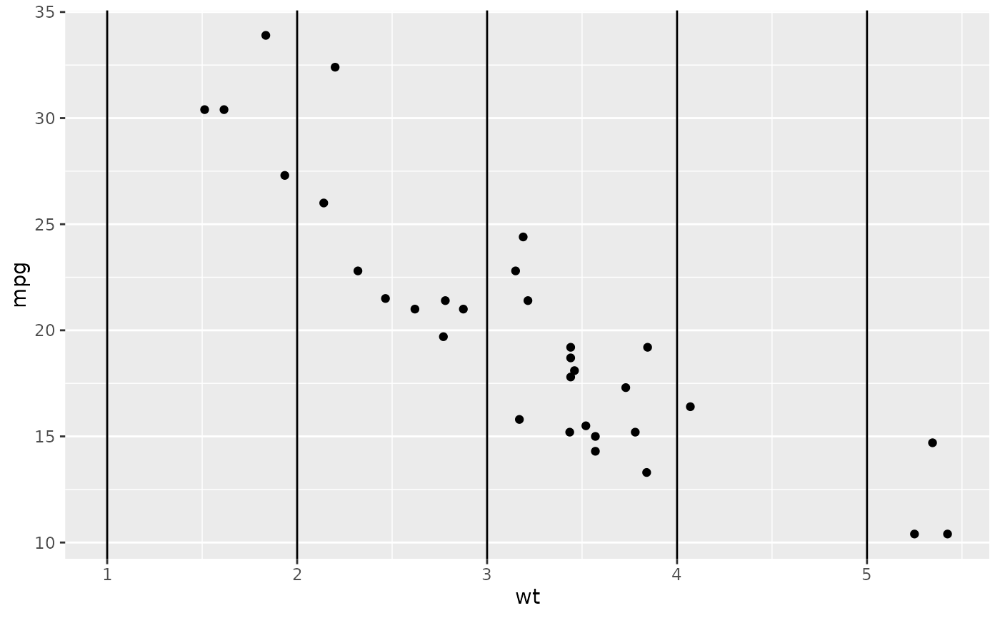
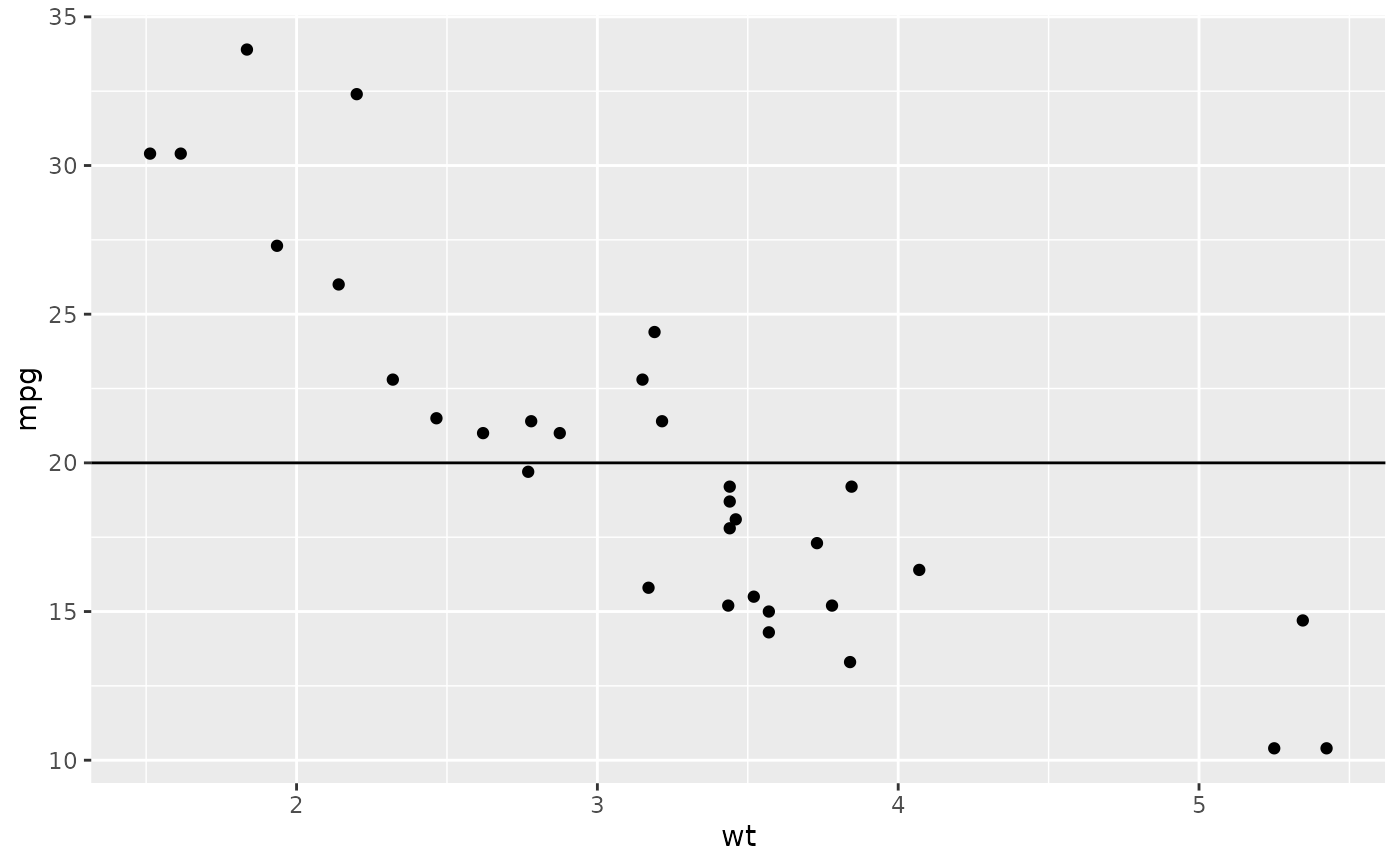
p <- ggplot(mtcars, aes(wt, mpg)) + geom_point()

# Fixed values
p + geom_vline(xintercept = 5)

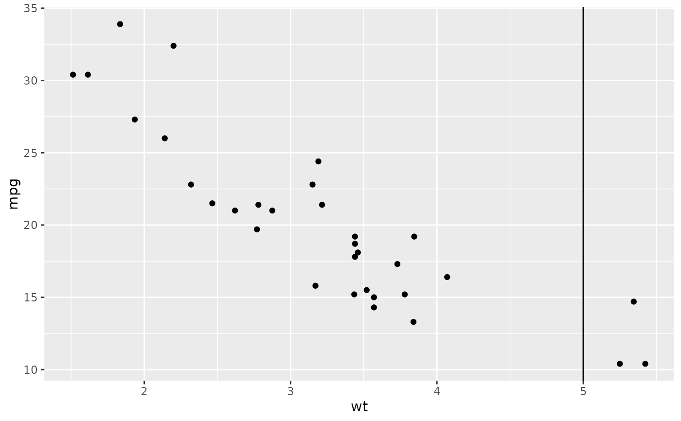p + geom_vline(xintercept = 1:5)

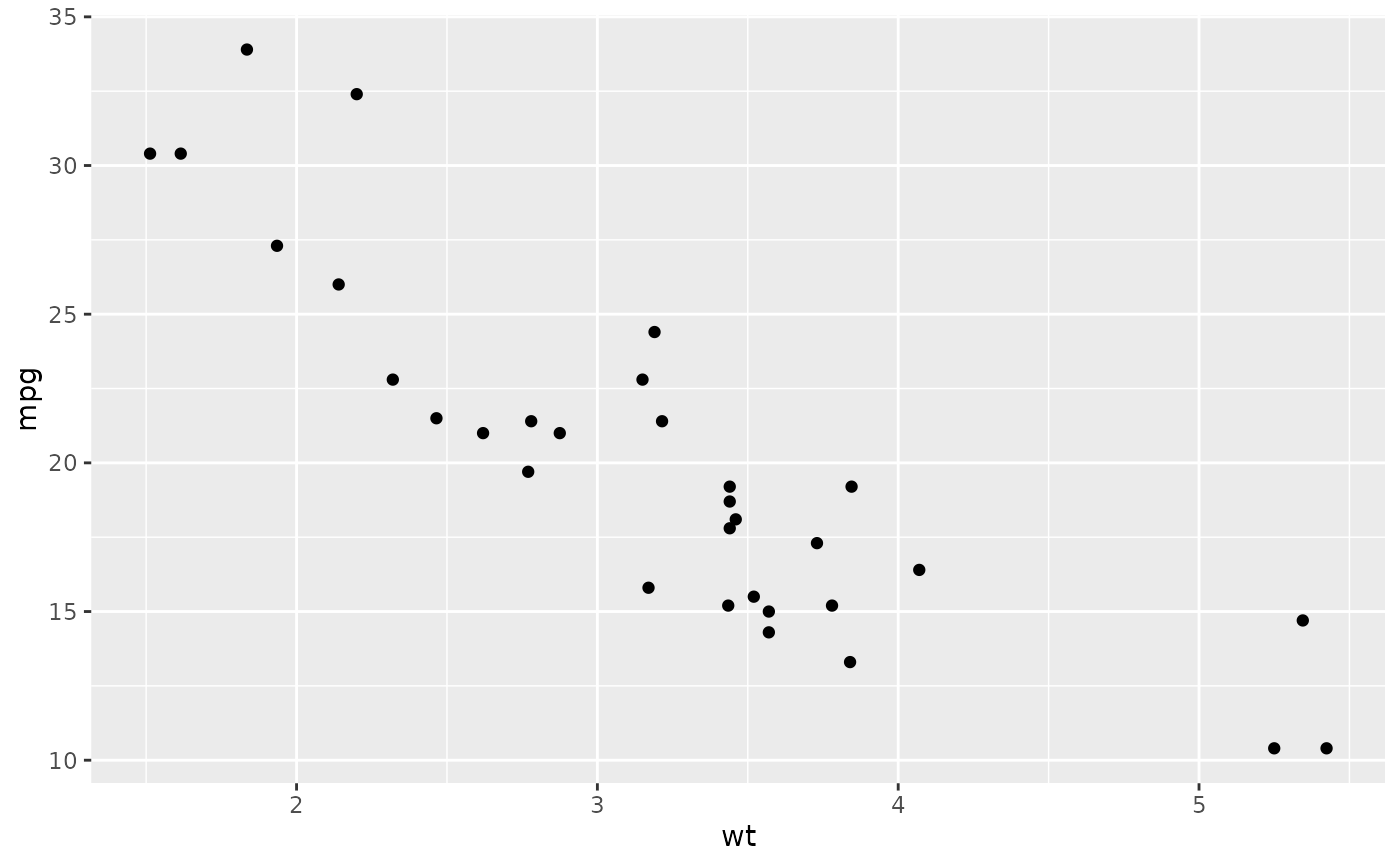
p + geom_hline(yintercept = 20)


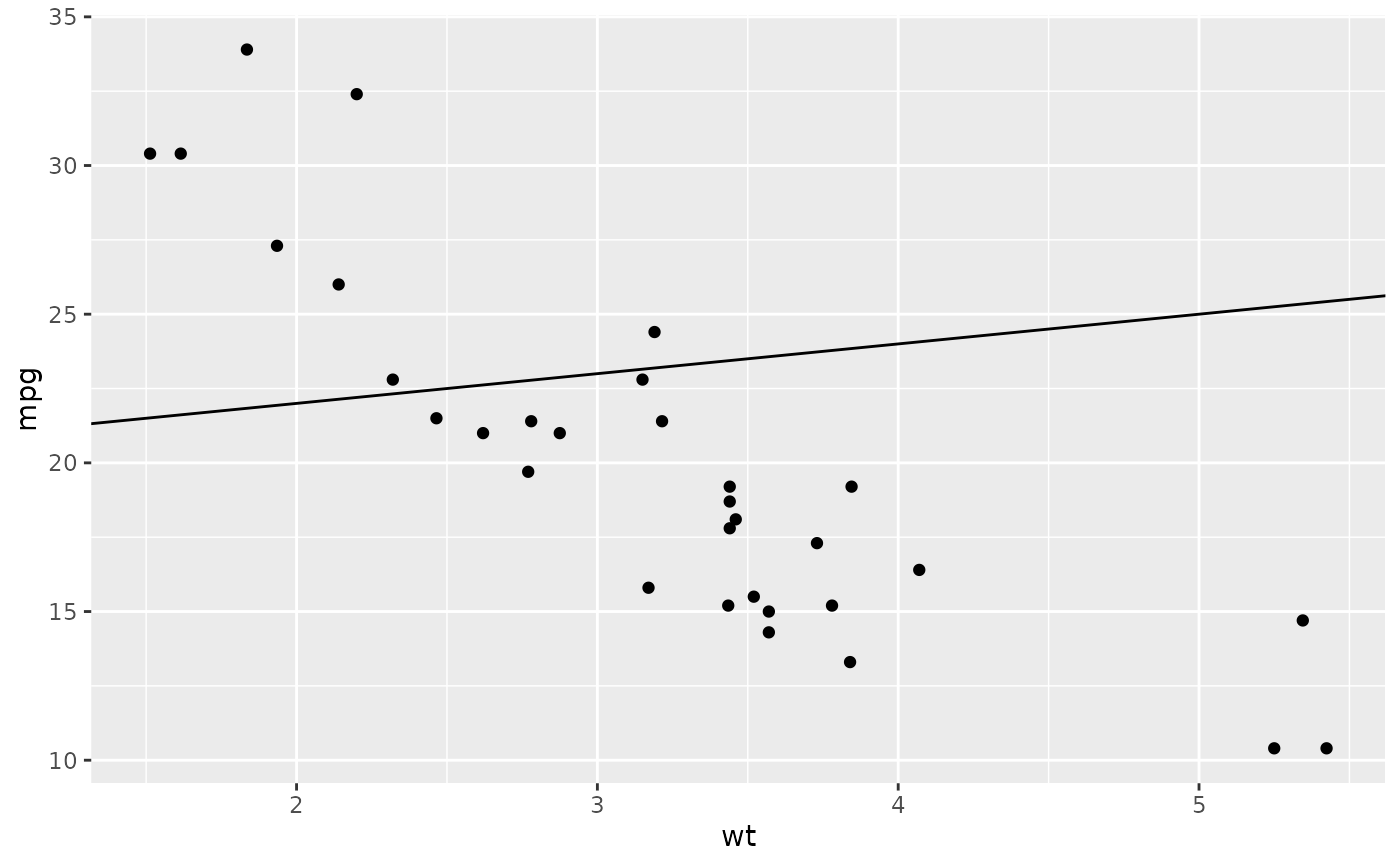
p + geom_abline() # Can't see it - outside the range of the data

p + geom_abline(intercept = 20)


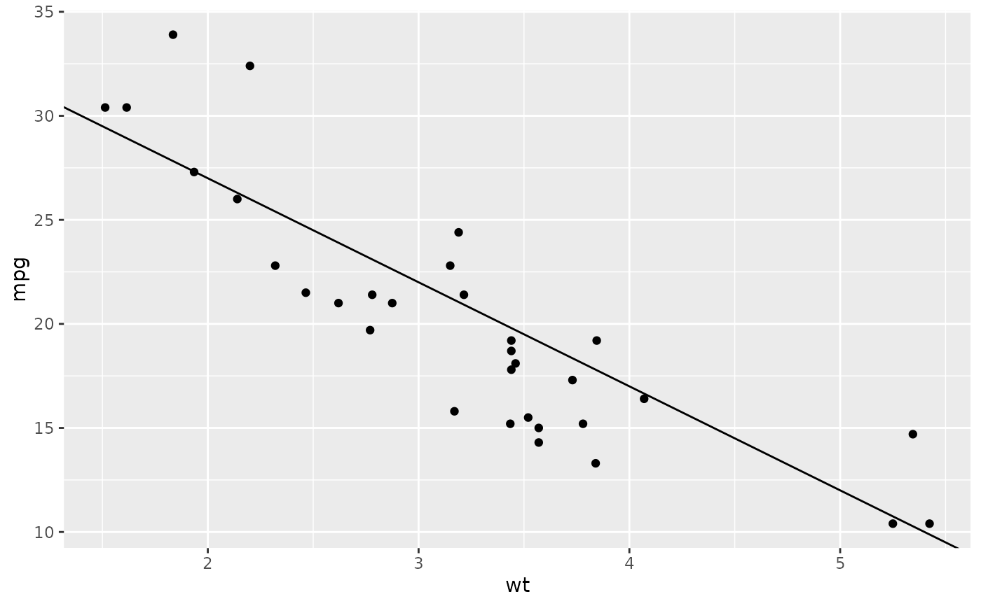
# Calculate slope and intercept of line of best fit
coef(lm(mpg ~ wt, data = mtcars))
#> (Intercept)          wt 
#>   37.285126   -5.344472 
p + geom_abline(intercept = 37, slope = -5)

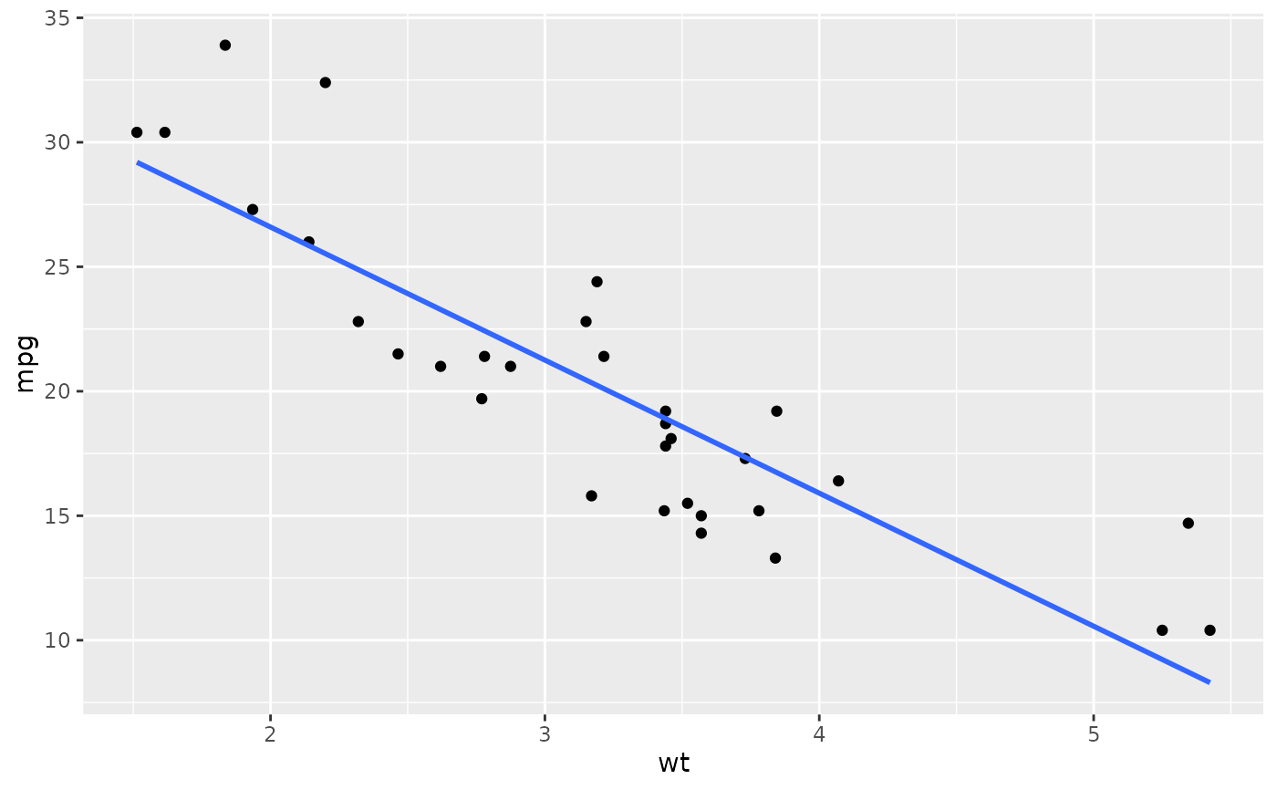
# But this is easier to do with geom_smooth:
p + geom_smooth(method = "lm", se = FALSE)
#> `geom_smooth()` using formula = 'y ~ x'


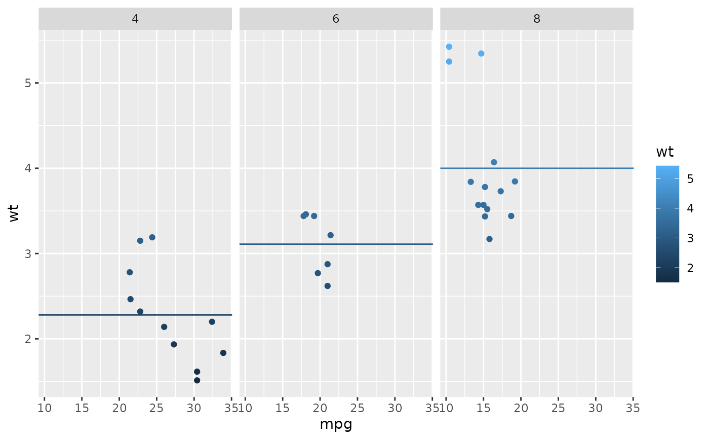
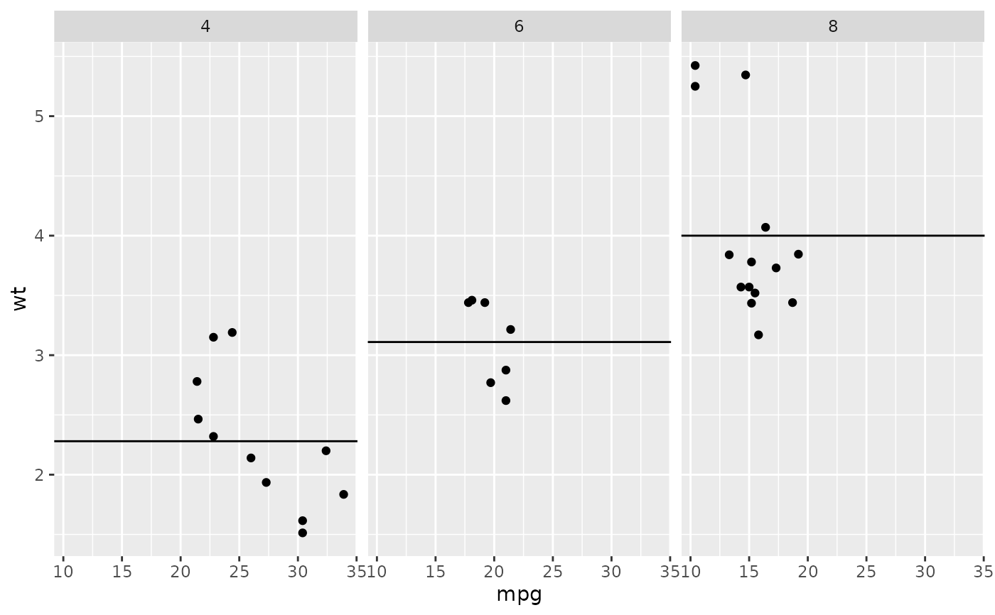
# To show different lines in different facets, use aesthetics
p <- ggplot(mtcars, aes(mpg, wt)) +
  geom_point() +
  facet_wrap(~ cyl)

mean_wt <- data.frame(cyl = c(4, 6, 8), wt = c(2.28, 3.11, 4.00))
p + geom_hline(aes(yintercept = wt), mean_wt)


# You can also control other aesthetics
ggplot(mtcars, aes(mpg, wt, colour = wt)) +
  geom_point() +
  geom_hline(aes(yintercept = wt, colour = wt), mean_wt) +
  facet_wrap(~ cyl)