Extract coordinates from 'sf' objects

stat_sf_coordinates() extracts the coordinates from 'sf' objects and summarises them to one pair of coordinates (x and y) per geometry. This is convenient when you draw an sf object as geoms like text and labels (so geom_sf_text() and geom_sf_label() relies on this).

Usage

stat_sf_coordinates(
  mapping = aes(),
  data = NULL,
  geom = "point",
  position = "identity",
  na.rm = FALSE,
  show.legend = NA,
  inherit.aes = TRUE,
  fun.geometry = NULL,
  ...
)

Arguments

mapping

Set of aesthetic mappings created by aes(). If specified and inherit.aes = TRUE (the default), it is combined with the default mapping at the top level of the plot. You must supply mapping if there is no plot mapping.

data

The data to be displayed in this layer. There are three options:

If NULL, the default, the data is inherited from the plot data as specified in the call to ggplot().

A data.frame, or other object, will override the plot data. All objects will be fortified to produce a data frame. See fortify() for which variables will be created.

A function will be called with a single argument, the plot data. The return value must be a data.frame, and will be used as the layer data. A function can be created from a formula (e.g. ~ head(.x, 10)).

geom

The geometric object to use to display the data for this layer. When using a stat_*() function to construct a layer, the geom argument can be used to override the default coupling between stats and geoms. The geom argument accepts the following:

• A Geom ggproto subclass, for example GeomPoint.

• A string naming the geom. To give the geom as a string, strip the function name of the geom_ prefix. For example, to use geom_point(), give the geom as "point".

• For more information and other ways to specify the geom, see the layer geom documentation.

position

A position adjustment to use on the data for this layer. This can be used in various ways, including to prevent overplotting and improving the display. The position argument accepts the following:

• The result of calling a position function, such as position_jitter(). This method allows for passing extra arguments to the position.

• A string naming the position adjustment. To give the position as a string, strip the function name of the position_ prefix. For example, to use position_jitter(), give the position as "jitter".

• For more information and other ways to specify the position, see the layer position documentation.

na.rm

If FALSE, the default, missing values are removed with a warning. If TRUE, missing values are silently removed.

show.legend

logical. Should this layer be included in the legends? NA, the default, includes if any aesthetics are mapped. FALSE never includes, and TRUE always includes. It can also be a named logical vector to finely select the aesthetics to display.

inherit.aes

If FALSE, overrides the default aesthetics, rather than combining with them. This is most useful for helper functions that define both data and aesthetics and shouldn't inherit behaviour from the default plot specification, e.g. borders().

fun.geometry

A function that takes a sfc object and returns a sfc_POINT with the same length as the input. If NULL, function(x) sf::st_point_on_surface(sf::st_zm(x)) will be used. Note that the function may warn about the incorrectness of the result if the data is not projected, but you can ignore this except when you really care about the exact locations.

...

Other arguments passed on to layer()'s params argument. These arguments broadly fall into one of 4 categories below. Notably, further arguments to the position argument, or aesthetics that are required can not be passed through .... Unknown arguments that are not part of the 4 categories below are ignored.

• Static aesthetics that are not mapped to a scale, but are at a fixed value and apply to the layer as a whole. For example, colour = "red" or linewidth = 3. The geom's documentation has an Aesthetics section that lists the available options. The 'required' aesthetics cannot be passed on to the params. Please note that while passing unmapped aesthetics as vectors is technically possible, the order and required length is not guaranteed to be parallel to the input data.

• When constructing a layer using a stat_*() function, the ... argument can be used to pass on parameters to the geom part of the layer. An example of this is stat_density(geom = "area", outline.type = "both"). The geom's documentation lists which parameters it can accept.

• Inversely, when constructing a layer using a geom_*() function, the ... argument can be used to pass on parameters to the stat part of the layer. An example of this is geom_area(stat = "density", adjust = 0.5). The stat's documentation lists which parameters it can accept.

• The key_glyph argument of layer() may also be passed on through .... This can be one of the functions described as key glyphs, to change the display of the layer in the legend.

Details

coordinates of an sf object can be retrieved by sf::st_coordinates(). But, we cannot simply use sf::st_coordinates() because, whereas text and labels require exactly one coordinate per geometry, it returns multiple ones for a polygon or a line. Thus, these two steps are needed:

1. Choose one point per geometry by some function like sf::st_centroid() or sf::st_point_on_surface().

2. Retrieve coordinates from the points by sf::st_coordinates().

For the first step, you can use an arbitrary function via fun.geometry. By default, function(x) sf::st_point_on_surface(sf::st_zm(x)) is used; sf::st_point_on_surface() seems more appropriate than sf::st_centroid() since labels and text usually are intended to be put within the polygon or the line. sf::st_zm() is needed to drop Z and M dimension beforehand, otherwise sf::st_point_on_surface() may fail when the geometries have M dimension.

Computed variables

These are calculated by the 'stat' part of layers and can be accessed with delayed evaluation.

• after_stat(x)
  X dimension of the simple feature.

• after_stat(y)
  Y dimension of the simple feature.

Examples

if (requireNamespace("sf", quietly = TRUE)) {
nc <- sf::st_read(system.file("shape/nc.shp", package="sf"))

ggplot(nc) +
  stat_sf_coordinates()

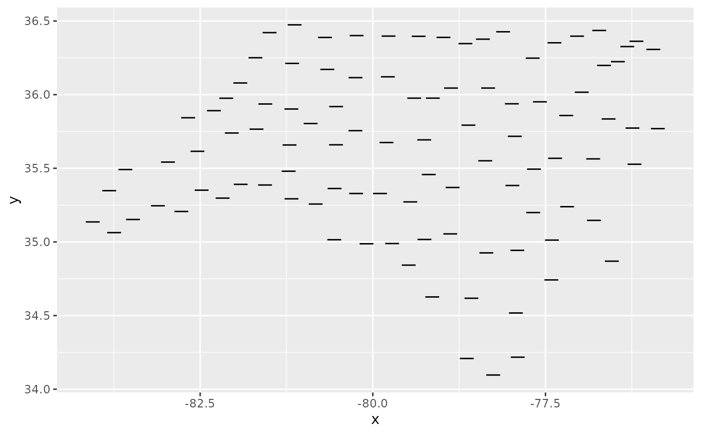
ggplot(nc) +
  geom_errorbarh(
    aes(geometry = geometry,
        xmin = after_stat(x) - 0.1,
        xmax = after_stat(x) + 0.1,
        y = after_stat(y),
        height = 0.04),
    stat = "sf_coordinates"
  )
}
#> Reading layer `nc' from data source 
#>   `/home/runner/work/_temp/Library/sf/shape/nc.shp' 
#>   using driver `ESRI Shapefile'
#> Simple feature collection with 100 features and 14 fields
#> Geometry type: MULTIPOLYGON
#> Dimension:     XY
#> Bounding box:  xmin: -84.32385 ymin: 33.88199 xmax: -75.45698 ymax: 36.58965
#> Geodetic CRS:  NAD27
#> Warning: st_point_on_surface may not give correct results for longitude/latitude data