geom_qq() and stat_qq() produce quantile-quantile plots. geom_qq_line() and
stat_qq_line() compute the slope and intercept of the line connecting the
points at specified quartiles of the theoretical and sample distributions.
Usage
geom_qq_line(
  mapping = NULL,
  data = NULL,
  geom = "abline",
  position = "identity",
  ...,
  distribution = stats::qnorm,
  dparams = list(),
  line.p = c(0.25, 0.75),
  fullrange = FALSE,
  na.rm = FALSE,
  show.legend = NA,
  inherit.aes = TRUE
)

stat_qq_line(
  mapping = NULL,
  data = NULL,
  geom = "abline",
  position = "identity",
  ...,
  distribution = stats::qnorm,
  dparams = list(),
  line.p = c(0.25, 0.75),
  fullrange = FALSE,
  na.rm = FALSE,
  show.legend = NA,
  inherit.aes = TRUE
)

geom_qq(
  mapping = NULL,
  data = NULL,
  geom = "point",
  position = "identity",
  ...,
  distribution = stats::qnorm,
  dparams = list(),
  na.rm = FALSE,
  show.legend = NA,
  inherit.aes = TRUE
)

stat_qq(
  mapping = NULL,
  data = NULL,
  geom = "point",
  position = "identity",
  ...,
  distribution = stats::qnorm,
  dparams = list(),
  na.rm = FALSE,
  show.legend = NA,
  inherit.aes = TRUE
)
Arguments
- mapping
Set of aesthetic mappings created by
aes(). If specified andinherit.aes = TRUE(the default), it is combined with the default mapping at the top level of the plot. You must supplymappingif there is no plot mapping.- data
The data to be displayed in this layer. There are three options:
If
NULL, the default, the data is inherited from the plot data as specified in the call toggplot().A
data.frame, or other object, will override the plot data. All objects will be fortified to produce a data frame. Seefortify()for which variables will be created.A
functionwill be called with a single argument, the plot data. The return value must be adata.frame, and will be used as the layer data. Afunctioncan be created from aformula(e.g.~ head(.x, 10)).- geom
The geometric object to use to display the data for this layer. When using a
stat_*()function to construct a layer, thegeomargument can be used to override the default coupling between stats and geoms. Thegeomargument accepts the following:A
Geomggproto subclass, for exampleGeomPoint.A string naming the geom. To give the geom as a string, strip the function name of the
geom_prefix. For example, to usegeom_point(), give the geom as"point".For more information and other ways to specify the geom, see the layer geom documentation.
- position
A position adjustment to use on the data for this layer. This can be used in various ways, including to prevent overplotting and improving the display. The
positionargument accepts the following:The result of calling a position function, such as
position_jitter(). This method allows for passing extra arguments to the position.A string naming the position adjustment. To give the position as a string, strip the function name of the
position_prefix. For example, to useposition_jitter(), give the position as"jitter".For more information and other ways to specify the position, see the layer position documentation.
- ...
Other arguments passed on to
layer()'sparamsargument. These arguments broadly fall into one of 4 categories below. Notably, further arguments to thepositionargument, or aesthetics that are required can not be passed through.... Unknown arguments that are not part of the 4 categories below are ignored.Static aesthetics that are not mapped to a scale, but are at a fixed value and apply to the layer as a whole. For example,
colour = "red"orlinewidth = 3. The geom's documentation has an Aesthetics section that lists the available options. The 'required' aesthetics cannot be passed on to theparams. Please note that while passing unmapped aesthetics as vectors is technically possible, the order and required length is not guaranteed to be parallel to the input data.When constructing a layer using a
stat_*()function, the...argument can be used to pass on parameters to thegeompart of the layer. An example of this isstat_density(geom = "area", outline.type = "both"). The geom's documentation lists which parameters it can accept.Inversely, when constructing a layer using a
geom_*()function, the...argument can be used to pass on parameters to thestatpart of the layer. An example of this isgeom_area(stat = "density", adjust = 0.5). The stat's documentation lists which parameters it can accept.The
key_glyphargument oflayer()may also be passed on through.... This can be one of the functions described as key glyphs, to change the display of the layer in the legend.
- distribution
Distribution function to use, if x not specified
- dparams
Additional parameters passed on to
distributionfunction.- line.p
Vector of quantiles to use when fitting the Q-Q line, defaults defaults to
c(.25, .75).- fullrange
Should the q-q line span the full range of the plot, or just the data
- na.rm
If
FALSE, the default, missing values are removed with a warning. IfTRUE, missing values are silently removed.- show.legend
logical. Should this layer be included in the legends?
NA, the default, includes if any aesthetics are mapped.FALSEnever includes, andTRUEalways includes. It can also be a named logical vector to finely select the aesthetics to display. To include legend keys for all levels, even when no data exists, useTRUE. IfNA, all levels are shown in legend, but unobserved levels are omitted.- inherit.aes
If
FALSE, overrides the default aesthetics, rather than combining with them. This is most useful for helper functions that define both data and aesthetics and shouldn't inherit behaviour from the default plot specification, e.g.annotation_borders().
Computed variables
These are calculated by the 'stat' part of layers and can be accessed with delayed evaluation.
Variables computed by stat_qq():
after_stat(sample)
Sample quantiles.after_stat(theoretical)
Theoretical quantiles.
Variables computed by stat_qq_line():
after_stat(x)
x-coordinates of the endpoints of the line segment connecting the points at the chosen quantiles of the theoretical and the sample distributions.after_stat(y)
y-coordinates of the endpoints.after_stat(slope)
Amount of change inyacross 1 unit ofx.after_stat(intercept)
Value ofyatx == 0.
Aesthetics
stat_qq() understands the following aesthetics. Required aesthetics are displayed in bold and defaults are displayed for optional aesthetics:
| • | sample | |
| • | group | → inferred |
| • | x | → after_stat(theoretical) |
| • | y | → after_stat(sample) |
stat_qq_line() understands the following aesthetics. Required aesthetics are displayed in bold and defaults are displayed for optional aesthetics:
| • | sample | |
| • | group | → inferred |
| • | x | → after_stat(x) |
| • | y | → after_stat(y) |
Learn more about setting these aesthetics in vignette("ggplot2-specs").
Examples
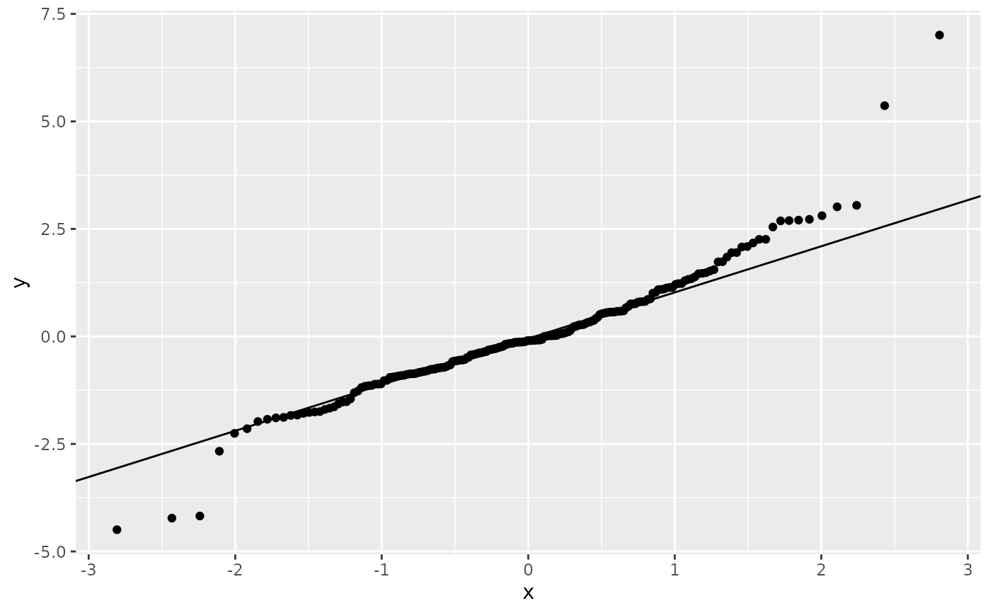
# \donttest{
df <- data.frame(y = rt(200, df = 5))
p <- ggplot(df, aes(sample = y))
p + stat_qq() + stat_qq_line()
 # Use fitdistr from MASS to estimate distribution params:
# if (requireNamespace("MASS", quietly = TRUE)) {
# params <- as.list(MASS::fitdistr(df$y, "t")$estimate)
# }
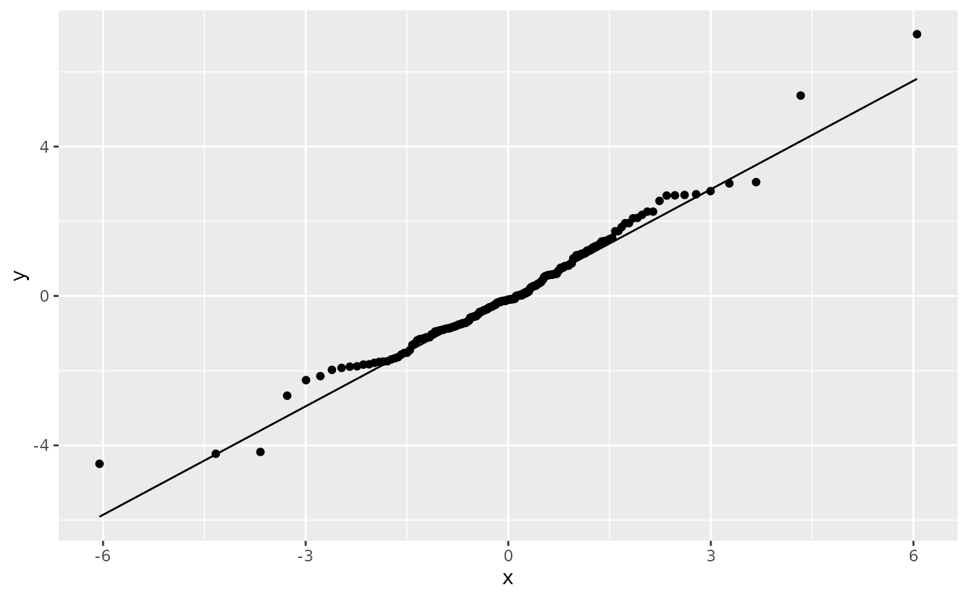
# Here, we use pre-computed params
params <- list(m = -0.02505057194115, s = 1.122568610124, df = 6.63842653897)
ggplot(df, aes(sample = y)) +
stat_qq(distribution = qt, dparams = params["df"]) +
stat_qq_line(distribution = qt, dparams = params["df"])
# Use fitdistr from MASS to estimate distribution params:
# if (requireNamespace("MASS", quietly = TRUE)) {
# params <- as.list(MASS::fitdistr(df$y, "t")$estimate)
# }
# Here, we use pre-computed params
params <- list(m = -0.02505057194115, s = 1.122568610124, df = 6.63842653897)
ggplot(df, aes(sample = y)) +
stat_qq(distribution = qt, dparams = params["df"]) +
stat_qq_line(distribution = qt, dparams = params["df"])
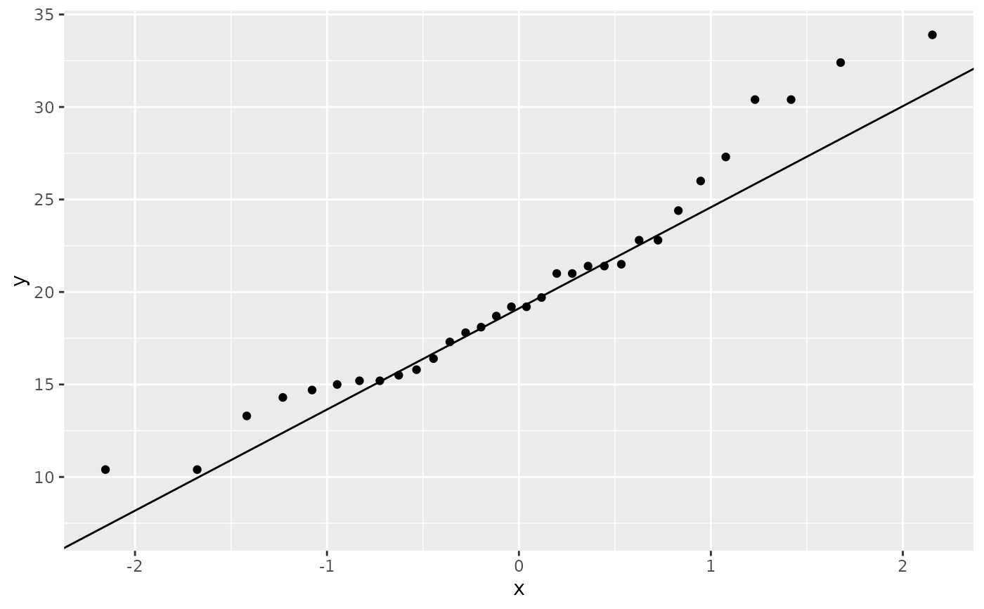
 # Using to explore the distribution of a variable
ggplot(mtcars, aes(sample = mpg)) +
stat_qq() +
stat_qq_line()
# Using to explore the distribution of a variable
ggplot(mtcars, aes(sample = mpg)) +
stat_qq() +
stat_qq_line()
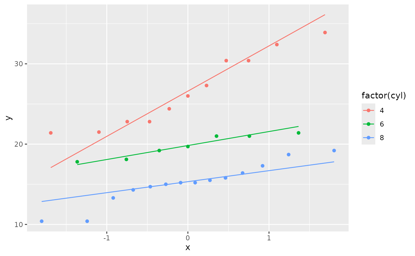
 ggplot(mtcars, aes(sample = mpg, colour = factor(cyl))) +
stat_qq() +
stat_qq_line()
ggplot(mtcars, aes(sample = mpg, colour = factor(cyl))) +
stat_qq() +
stat_qq_line()
 # }
# }