# ggplot2
## Overview
ggplot2 is a system for declaratively creating graphics, based on [The
Grammar of
Graphics](https://link.springer.com/book/10.1007/0-387-28695-0). You
provide the data, tell ggplot2 how to map variables to aesthetics, what
graphical primitives to use, and it takes care of the details.
## Installation
``` r
# The easiest way to get ggplot2 is to install the whole tidyverse:
install.packages("tidyverse")
# Alternatively, install just ggplot2:
install.packages("ggplot2")
# Or the development version from GitHub:
# install.packages("pak")
pak::pak("tidyverse/ggplot2")
```
## Cheatsheet
[](https://github.com/rstudio/cheatsheets/blob/master/data-visualization.pdf)
## Usage
It’s hard to succinctly describe how ggplot2 works because it embodies a
deep philosophy of visualisation. However, in most cases you start with
[`ggplot()`](https://ggplot2.tidyverse.org/reference/ggplot.md), supply
a dataset and aesthetic mapping (with
[`aes()`](https://ggplot2.tidyverse.org/reference/aes.md)). You then add
on layers (like
[`geom_point()`](https://ggplot2.tidyverse.org/reference/geom_point.md)
or
[`geom_histogram()`](https://ggplot2.tidyverse.org/reference/geom_histogram.md)),
scales (like
[`scale_colour_brewer()`](https://ggplot2.tidyverse.org/reference/scale_brewer.md)),
faceting specifications (like
[`facet_wrap()`](https://ggplot2.tidyverse.org/reference/facet_wrap.md))
and coordinate systems (like
[`coord_flip()`](https://ggplot2.tidyverse.org/reference/coord_flip.md)).
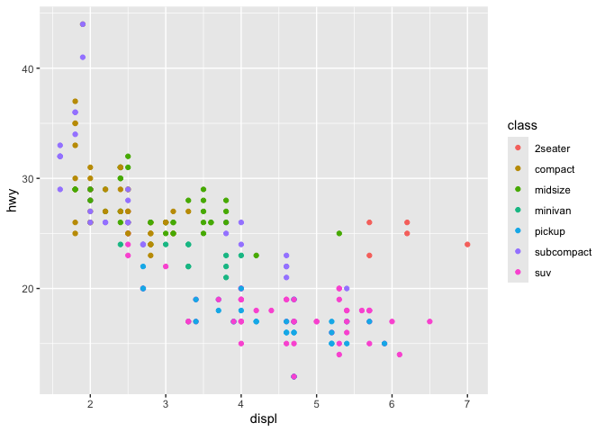
``` r
library(ggplot2)
ggplot(mpg, aes(displ, hwy, colour = class)) +
geom_point()
```
## Lifecycle
[](https://lifecycle.r-lib.org/articles/stages.html)
ggplot2 is now over 10 years old and is used by hundreds of thousands of
people to make millions of plots. That means, by-and-large, ggplot2
itself changes relatively little. When we do make changes, they will be
generally to add new functions or arguments rather than changing the
behaviour of existing functions, and if we do make changes to existing
behaviour we will do them for compelling reasons.
If you are looking for innovation, look to ggplot2’s rich ecosystem of
extensions. See a community maintained list at
.
## Learning ggplot2
If you are new to ggplot2 you are better off starting with a systematic
introduction, rather than trying to learn from reading individual
documentation pages. Currently, there are several good places to start:
1. The [Data Visualization](https://r4ds.hadley.nz/data-visualize) and
[Communication](https://r4ds.hadley.nz/communication) chapters in [R
for Data Science](https://r4ds.hadley.nz). R for Data Science is
designed to give you a comprehensive introduction to the
[tidyverse](https://tidyverse.org/), and these two chapters will get
you up to speed with the essentials of ggplot2 as quickly as
possible.
2. If you’d like to take an online course, try [Data Visualization in R
With
ggplot2](https://learning.oreilly.com/videos/data-visualization-in/9781491963661/)
by Kara Woo.
3. If you’d like to follow a webinar, try [Plotting Anything with
ggplot2](https://youtu.be/h29g21z0a68) by Thomas Lin Pedersen.
4. If you want to dive into making common graphics as quickly as
possible, I recommend [The R Graphics
Cookbook](https://r-graphics.org) by Winston Chang. It provides a
set of recipes to solve common graphics problems.
5. If you’ve mastered the basics and want to learn more, read [ggplot2:
Elegant Graphics for Data Analysis](https://ggplot2-book.org). It
describes the theoretical underpinnings of ggplot2 and shows you how
all the pieces fit together. This book helps you understand the
theory that underpins ggplot2, and will help you create new types of
graphics specifically tailored to your needs.
6. For articles about announcements and deep-dives you can visit the
[tidyverse blog](https://tidyverse.org/tags/ggplot2/).
## Getting help
There are two main places to get help with ggplot2:
1. The [Posit Community](https://forum.posit.co/) (formerly RStudio
Community) is a friendly place to ask any questions about ggplot2.
2. [Stack
Overflow](https://stackoverflow.com/questions/tagged/ggplot2?sort=frequent&pageSize=50)
is a great source of answers to common ggplot2 questions. It is also
a great place to get help, once you have created a reproducible
example that illustrates your problem.
# Package index
## Plot basics
All ggplot2 plots begin with a call to
[`ggplot()`](https://ggplot2.tidyverse.org/reference/ggplot.md),
supplying default data and aesthetic mappings, specified by
[`aes()`](https://ggplot2.tidyverse.org/reference/aes.md). You then add
layers, scales, coords and facets with `+`. To save a plot to disk, use
[`ggsave()`](https://ggplot2.tidyverse.org/reference/ggsave.md).
- [`ggplot()`](https://ggplot2.tidyverse.org/reference/ggplot.md) :
Create a new ggplot
- [`aes()`](https://ggplot2.tidyverse.org/reference/aes.md) : Construct
aesthetic mappings
- [`add_gg()`](https://ggplot2.tidyverse.org/reference/gg-add.md)
[`` `%+%` ``](https://ggplot2.tidyverse.org/reference/gg-add.md) : Add
components to a plot
- [`ggsave()`](https://ggplot2.tidyverse.org/reference/ggsave.md) : Save
a ggplot (or other grid object) with sensible defaults
- [`qplot()`](https://ggplot2.tidyverse.org/reference/qplot.md)
[`quickplot()`](https://ggplot2.tidyverse.org/reference/qplot.md) :
Quick plot
## Layers
### Geoms
A layer combines data, aesthetic mapping, a geom (geometric object), a
stat (statistical transformation), and a position adjustment. Typically,
you will create layers using a `geom_` function, overriding the default
position and stat if needed.
- [`layer_geoms`](https://ggplot2.tidyverse.org/reference/layer_geoms.md)
: Layer geometry display
- [](https://ggplot2.tidyverse.org/reference/geom_abline.md)
[`geom_abline()`](https://ggplot2.tidyverse.org/reference/geom_abline.md)
[`geom_hline()`](https://ggplot2.tidyverse.org/reference/geom_abline.md)
[`geom_vline()`](https://ggplot2.tidyverse.org/reference/geom_abline.md)
: Reference lines: horizontal, vertical, and diagonal
- [](https://ggplot2.tidyverse.org/reference/geom_bar.md)
[`geom_bar()`](https://ggplot2.tidyverse.org/reference/geom_bar.md)
[`geom_col()`](https://ggplot2.tidyverse.org/reference/geom_bar.md)
[`stat_count()`](https://ggplot2.tidyverse.org/reference/geom_bar.md)
: Bar charts
- [](https://ggplot2.tidyverse.org/reference/geom_bin_2d.md)
[`geom_bin_2d()`](https://ggplot2.tidyverse.org/reference/geom_bin_2d.md)
[`stat_bin_2d()`](https://ggplot2.tidyverse.org/reference/geom_bin_2d.md)
: Heatmap of 2d bin counts
- [](https://ggplot2.tidyverse.org/reference/geom_blank.md)
[`geom_blank()`](https://ggplot2.tidyverse.org/reference/geom_blank.md)
: Draw nothing
- [](https://ggplot2.tidyverse.org/reference/geom_boxplot.md)
[`geom_boxplot()`](https://ggplot2.tidyverse.org/reference/geom_boxplot.md)
[`stat_boxplot()`](https://ggplot2.tidyverse.org/reference/geom_boxplot.md)
: A box and whiskers plot (in the style of Tukey)
- [](https://ggplot2.tidyverse.org/reference/geom_contour.md)
[`geom_contour()`](https://ggplot2.tidyverse.org/reference/geom_contour.md)
[`geom_contour_filled()`](https://ggplot2.tidyverse.org/reference/geom_contour.md)
[`stat_contour()`](https://ggplot2.tidyverse.org/reference/geom_contour.md)
[`stat_contour_filled()`](https://ggplot2.tidyverse.org/reference/geom_contour.md)
: 2D contours of a 3D surface
- [](https://ggplot2.tidyverse.org/reference/geom_count.md)
[`geom_count()`](https://ggplot2.tidyverse.org/reference/geom_count.md)
[`stat_sum()`](https://ggplot2.tidyverse.org/reference/geom_count.md)
: Count overlapping points
- [](https://ggplot2.tidyverse.org/reference/geom_density.md)
[`geom_density()`](https://ggplot2.tidyverse.org/reference/geom_density.md)
[`stat_density()`](https://ggplot2.tidyverse.org/reference/geom_density.md)
: Smoothed density estimates
- [`geom_density_2d()`](https://ggplot2.tidyverse.org/reference/geom_density_2d.md)
[`geom_density_2d_filled()`](https://ggplot2.tidyverse.org/reference/geom_density_2d.md)
[`stat_density_2d()`](https://ggplot2.tidyverse.org/reference/geom_density_2d.md)
[`stat_density_2d_filled()`](https://ggplot2.tidyverse.org/reference/geom_density_2d.md)
: Contours of a 2D density estimate
- [](https://ggplot2.tidyverse.org/reference/geom_dotplot.md)
[`geom_dotplot()`](https://ggplot2.tidyverse.org/reference/geom_dotplot.md)
: Dot plot
- [`geom_function()`](https://ggplot2.tidyverse.org/reference/geom_function.md)
[`stat_function()`](https://ggplot2.tidyverse.org/reference/geom_function.md)
: Draw a function as a continuous curve
- [](https://ggplot2.tidyverse.org/reference/geom_hex.md)
[`geom_hex()`](https://ggplot2.tidyverse.org/reference/geom_hex.md)
[`stat_bin_hex()`](https://ggplot2.tidyverse.org/reference/geom_hex.md)
: Hexagonal heatmap of 2d bin counts
- [](https://ggplot2.tidyverse.org/reference/geom_histogram.md)
[`geom_freqpoly()`](https://ggplot2.tidyverse.org/reference/geom_histogram.md)
[`geom_histogram()`](https://ggplot2.tidyverse.org/reference/geom_histogram.md)
[`stat_bin()`](https://ggplot2.tidyverse.org/reference/geom_histogram.md)
: Histograms and frequency polygons
- [](https://ggplot2.tidyverse.org/reference/geom_jitter.md)
[`geom_jitter()`](https://ggplot2.tidyverse.org/reference/geom_jitter.md)
: Jittered points
- [](https://ggplot2.tidyverse.org/reference/geom_linerange.md)
[`geom_crossbar()`](https://ggplot2.tidyverse.org/reference/geom_linerange.md)
[`geom_errorbar()`](https://ggplot2.tidyverse.org/reference/geom_linerange.md)
[`geom_errorbarh()`](https://ggplot2.tidyverse.org/reference/geom_linerange.md)
[`geom_linerange()`](https://ggplot2.tidyverse.org/reference/geom_linerange.md)
[`geom_pointrange()`](https://ggplot2.tidyverse.org/reference/geom_linerange.md)
: Vertical intervals: lines, crossbars & errorbars
- [](https://ggplot2.tidyverse.org/reference/geom_map.md)
[`geom_map()`](https://ggplot2.tidyverse.org/reference/geom_map.md) :
Polygons from a reference map
- [](https://ggplot2.tidyverse.org/reference/geom_path.md)
[`geom_path()`](https://ggplot2.tidyverse.org/reference/geom_path.md)
[`geom_line()`](https://ggplot2.tidyverse.org/reference/geom_path.md)
[`geom_step()`](https://ggplot2.tidyverse.org/reference/geom_path.md)
: Connect observations
- [](https://ggplot2.tidyverse.org/reference/geom_point.md)
[`geom_point()`](https://ggplot2.tidyverse.org/reference/geom_point.md)
: Points
- [](https://ggplot2.tidyverse.org/reference/geom_polygon.md)
[`geom_polygon()`](https://ggplot2.tidyverse.org/reference/geom_polygon.md)
: Polygons
- [`geom_qq_line()`](https://ggplot2.tidyverse.org/reference/geom_qq.md)
[`stat_qq_line()`](https://ggplot2.tidyverse.org/reference/geom_qq.md)
[`geom_qq()`](https://ggplot2.tidyverse.org/reference/geom_qq.md)
[`stat_qq()`](https://ggplot2.tidyverse.org/reference/geom_qq.md) : A
quantile-quantile plot
- [](https://ggplot2.tidyverse.org/reference/geom_quantile.md)
[`geom_quantile()`](https://ggplot2.tidyverse.org/reference/geom_quantile.md)
[`stat_quantile()`](https://ggplot2.tidyverse.org/reference/geom_quantile.md)
: Quantile regression
- [](https://ggplot2.tidyverse.org/reference/geom_ribbon.md)
[`geom_ribbon()`](https://ggplot2.tidyverse.org/reference/geom_ribbon.md)
[`geom_area()`](https://ggplot2.tidyverse.org/reference/geom_ribbon.md)
[`stat_align()`](https://ggplot2.tidyverse.org/reference/geom_ribbon.md)
: Ribbons and area plots
- [](https://ggplot2.tidyverse.org/reference/geom_rug.md)
[`geom_rug()`](https://ggplot2.tidyverse.org/reference/geom_rug.md) :
Rug plots in the margins
- [](https://ggplot2.tidyverse.org/reference/geom_segment.md)
[`geom_segment()`](https://ggplot2.tidyverse.org/reference/geom_segment.md)
[`geom_curve()`](https://ggplot2.tidyverse.org/reference/geom_segment.md)
: Line segments and curves
- [](https://ggplot2.tidyverse.org/reference/geom_smooth.md)
[`geom_smooth()`](https://ggplot2.tidyverse.org/reference/geom_smooth.md)
[`stat_smooth()`](https://ggplot2.tidyverse.org/reference/geom_smooth.md)
: Smoothed conditional means
- [](https://ggplot2.tidyverse.org/reference/geom_spoke.md)
[`geom_spoke()`](https://ggplot2.tidyverse.org/reference/geom_spoke.md)
: Line segments parameterised by location, direction and distance
- [](https://ggplot2.tidyverse.org/reference/geom_text.md)
[`geom_label()`](https://ggplot2.tidyverse.org/reference/geom_text.md)
[`geom_text()`](https://ggplot2.tidyverse.org/reference/geom_text.md)
: Text
- [](https://ggplot2.tidyverse.org/reference/geom_tile.md)
[`geom_raster()`](https://ggplot2.tidyverse.org/reference/geom_tile.md)
[`geom_rect()`](https://ggplot2.tidyverse.org/reference/geom_tile.md)
[`geom_tile()`](https://ggplot2.tidyverse.org/reference/geom_tile.md)
: Rectangles
- [](https://ggplot2.tidyverse.org/reference/geom_violin.md)
[`geom_violin()`](https://ggplot2.tidyverse.org/reference/geom_violin.md)
[`stat_ydensity()`](https://ggplot2.tidyverse.org/reference/geom_violin.md)
: Violin plot
- [](https://ggplot2.tidyverse.org/reference/ggsf.md)
[`coord_sf()`](https://ggplot2.tidyverse.org/reference/ggsf.md)
[`geom_sf()`](https://ggplot2.tidyverse.org/reference/ggsf.md)
[`geom_sf_label()`](https://ggplot2.tidyverse.org/reference/ggsf.md)
[`geom_sf_text()`](https://ggplot2.tidyverse.org/reference/ggsf.md)
[`stat_sf()`](https://ggplot2.tidyverse.org/reference/ggsf.md) :
Visualise sf objects
### Stats
A handful of layers are more easily specified with a `stat_` function,
drawing attention to the statistical transformation rather than the
visual appearance. The computed variables can be mapped using
[`after_stat()`](https://ggplot2.tidyverse.org/reference/aes_eval.md).
- [`layer_stats`](https://ggplot2.tidyverse.org/reference/layer_stats.md)
: Layer statistical transformations
- [`stat_ecdf()`](https://ggplot2.tidyverse.org/reference/stat_ecdf.md)
: Compute empirical cumulative distribution
- [`stat_ellipse()`](https://ggplot2.tidyverse.org/reference/stat_ellipse.md)
: Compute normal data ellipses
- [`geom_function()`](https://ggplot2.tidyverse.org/reference/geom_function.md)
[`stat_function()`](https://ggplot2.tidyverse.org/reference/geom_function.md)
: Draw a function as a continuous curve
- [`stat_identity()`](https://ggplot2.tidyverse.org/reference/stat_identity.md)
: Leave data as is
- [`stat_summary_2d()`](https://ggplot2.tidyverse.org/reference/stat_summary_2d.md)
[`stat_summary_hex()`](https://ggplot2.tidyverse.org/reference/stat_summary_2d.md)
: Bin and summarise in 2d (rectangle & hexagons)
- [`stat_summary_bin()`](https://ggplot2.tidyverse.org/reference/stat_summary.md)
[`stat_summary()`](https://ggplot2.tidyverse.org/reference/stat_summary.md)
: Summarise y values at unique/binned x
- [`stat_unique()`](https://ggplot2.tidyverse.org/reference/stat_unique.md)
: Remove duplicates
- [`stat_sf_coordinates()`](https://ggplot2.tidyverse.org/reference/stat_sf_coordinates.md)
: Extract coordinates from 'sf' objects
- [`stat_manual()`](https://ggplot2.tidyverse.org/reference/stat_manual.md)
: Manually compute transformations
- [`stat_connect()`](https://ggplot2.tidyverse.org/reference/stat_connect.md)
: Connect observations
- [`after_stat()`](https://ggplot2.tidyverse.org/reference/aes_eval.md)
[`after_scale()`](https://ggplot2.tidyverse.org/reference/aes_eval.md)
[`from_theme()`](https://ggplot2.tidyverse.org/reference/aes_eval.md)
[`stage()`](https://ggplot2.tidyverse.org/reference/aes_eval.md) :
Control aesthetic evaluation
### Position adjustment
All layers have a position adjustment that resolves overlapping geoms.
Override the default by using the `position` argument to the `geom_` or
`stat_` function.
- [`layer_positions`](https://ggplot2.tidyverse.org/reference/layer_positions.md)
: Layer position adjustments
- [](https://ggplot2.tidyverse.org/reference/position_dodge.md)
[`position_dodge()`](https://ggplot2.tidyverse.org/reference/position_dodge.md)
[`position_dodge2()`](https://ggplot2.tidyverse.org/reference/position_dodge.md)
: Dodge overlapping objects side-to-side
- [](https://ggplot2.tidyverse.org/reference/position_identity.md)
[`position_identity()`](https://ggplot2.tidyverse.org/reference/position_identity.md)
: Don't adjust position
- [](https://ggplot2.tidyverse.org/reference/position_jitter.md)
[`position_jitter()`](https://ggplot2.tidyverse.org/reference/position_jitter.md)
: Jitter points to avoid overplotting
- [`position_jitterdodge()`](https://ggplot2.tidyverse.org/reference/position_jitterdodge.md)
: Simultaneously dodge and jitter
- [`position_nudge()`](https://ggplot2.tidyverse.org/reference/position_nudge.md)
: Nudge points a fixed distance
- [](https://ggplot2.tidyverse.org/reference/position_stack.md)
[`position_stack()`](https://ggplot2.tidyverse.org/reference/position_stack.md)
[`position_fill()`](https://ggplot2.tidyverse.org/reference/position_stack.md)
: Stack overlapping objects on top of each another
### Annotations
Annotations are a special type of layer that don’t inherit global
settings from the plot. They are used to add fixed reference data to
plots.
- [](https://ggplot2.tidyverse.org/reference/geom_abline.md)
[`geom_abline()`](https://ggplot2.tidyverse.org/reference/geom_abline.md)
[`geom_hline()`](https://ggplot2.tidyverse.org/reference/geom_abline.md)
[`geom_vline()`](https://ggplot2.tidyverse.org/reference/geom_abline.md)
: Reference lines: horizontal, vertical, and diagonal
- [`annotate()`](https://ggplot2.tidyverse.org/reference/annotate.md) :
Create an annotation layer
- [`annotation_custom()`](https://ggplot2.tidyverse.org/reference/annotation_custom.md)
: Annotation: Custom grob
- [`annotation_logticks()`](https://ggplot2.tidyverse.org/reference/annotation_logticks.md)
**\[superseded\]** : Annotation: log tick marks
- [`annotation_map()`](https://ggplot2.tidyverse.org/reference/annotation_map.md)
: Annotation: a map
- [`annotation_raster()`](https://ggplot2.tidyverse.org/reference/annotation_raster.md)
: Annotation: high-performance rectangular tiling
- [`annotation_borders()`](https://ggplot2.tidyverse.org/reference/annotation_borders.md)
[`borders()`](https://ggplot2.tidyverse.org/reference/annotation_borders.md)
: Create a layer of map borders
## Aesthetics
The following help topics give a broad overview of some of the ways you
can use each aesthetic.
- [`aes_colour_fill_alpha`](https://ggplot2.tidyverse.org/reference/aes_colour_fill_alpha.md)
[`colour`](https://ggplot2.tidyverse.org/reference/aes_colour_fill_alpha.md)
[`color`](https://ggplot2.tidyverse.org/reference/aes_colour_fill_alpha.md)
[`fill`](https://ggplot2.tidyverse.org/reference/aes_colour_fill_alpha.md)
: Colour related aesthetics: colour, fill, and alpha
- [`aes_group_order`](https://ggplot2.tidyverse.org/reference/aes_group_order.md)
[`group`](https://ggplot2.tidyverse.org/reference/aes_group_order.md)
: Aesthetics: grouping
- [`aes_linetype_size_shape`](https://ggplot2.tidyverse.org/reference/aes_linetype_size_shape.md)
[`linetype`](https://ggplot2.tidyverse.org/reference/aes_linetype_size_shape.md)
[`size`](https://ggplot2.tidyverse.org/reference/aes_linetype_size_shape.md)
[`shape`](https://ggplot2.tidyverse.org/reference/aes_linetype_size_shape.md)
: Differentiation related aesthetics: linetype, size, shape
- [`aes_position`](https://ggplot2.tidyverse.org/reference/aes_position.md)
[`x`](https://ggplot2.tidyverse.org/reference/aes_position.md)
[`y`](https://ggplot2.tidyverse.org/reference/aes_position.md)
[`xmin`](https://ggplot2.tidyverse.org/reference/aes_position.md)
[`xmax`](https://ggplot2.tidyverse.org/reference/aes_position.md)
[`ymin`](https://ggplot2.tidyverse.org/reference/aes_position.md)
[`ymax`](https://ggplot2.tidyverse.org/reference/aes_position.md)
[`xend`](https://ggplot2.tidyverse.org/reference/aes_position.md)
[`yend`](https://ggplot2.tidyverse.org/reference/aes_position.md) :
Position related aesthetics: x, y, xmin, xmax, ymin, ymax, xend, yend
## Scales
Scales control the details of how data values are translated to visual
properties. Override the default scales to tweak details like the axis
labels or legend keys, or to use a completely different translation from
data to aesthetic.
[`labs()`](https://ggplot2.tidyverse.org/reference/labs.md) and
[`lims()`](https://ggplot2.tidyverse.org/reference/lims.md) are
convenient helpers for the most common adjustments to the labels and
limits.
- [`labs()`](https://ggplot2.tidyverse.org/reference/labs.md)
[`xlab()`](https://ggplot2.tidyverse.org/reference/labs.md)
[`ylab()`](https://ggplot2.tidyverse.org/reference/labs.md)
[`ggtitle()`](https://ggplot2.tidyverse.org/reference/labs.md)
[`get_labs()`](https://ggplot2.tidyverse.org/reference/labs.md)
**\[superseded\]** : Modify axis, legend, and plot labels
- [`lims()`](https://ggplot2.tidyverse.org/reference/lims.md)
[`xlim()`](https://ggplot2.tidyverse.org/reference/lims.md)
[`ylim()`](https://ggplot2.tidyverse.org/reference/lims.md) : Set
scale limits
- [`expand_limits()`](https://ggplot2.tidyverse.org/reference/expand_limits.md)
**\[superseded\]** : Expand the plot limits, using data
- [`expansion()`](https://ggplot2.tidyverse.org/reference/expansion.md)
[`expand_scale()`](https://ggplot2.tidyverse.org/reference/expansion.md)
: Generate expansion vector for scales
- [](https://ggplot2.tidyverse.org/reference/scale_alpha.md)
[`scale_alpha()`](https://ggplot2.tidyverse.org/reference/scale_alpha.md)
[`scale_alpha_continuous()`](https://ggplot2.tidyverse.org/reference/scale_alpha.md)
[`scale_alpha_binned()`](https://ggplot2.tidyverse.org/reference/scale_alpha.md)
[`scale_alpha_discrete()`](https://ggplot2.tidyverse.org/reference/scale_alpha.md)
[`scale_alpha_ordinal()`](https://ggplot2.tidyverse.org/reference/scale_alpha.md)
: Alpha transparency scales
- [`scale_x_binned()`](https://ggplot2.tidyverse.org/reference/scale_binned.md)
[`scale_y_binned()`](https://ggplot2.tidyverse.org/reference/scale_binned.md)
: Positional scales for binning continuous data (x & y)
- [](https://ggplot2.tidyverse.org/reference/scale_brewer.md)
[`scale_colour_brewer()`](https://ggplot2.tidyverse.org/reference/scale_brewer.md)
[`scale_fill_brewer()`](https://ggplot2.tidyverse.org/reference/scale_brewer.md)
[`scale_colour_distiller()`](https://ggplot2.tidyverse.org/reference/scale_brewer.md)
[`scale_fill_distiller()`](https://ggplot2.tidyverse.org/reference/scale_brewer.md)
[`scale_colour_fermenter()`](https://ggplot2.tidyverse.org/reference/scale_brewer.md)
[`scale_fill_fermenter()`](https://ggplot2.tidyverse.org/reference/scale_brewer.md)
: Sequential, diverging and qualitative colour scales from ColorBrewer
- [](https://ggplot2.tidyverse.org/reference/scale_colour_continuous.md)
[`scale_colour_continuous()`](https://ggplot2.tidyverse.org/reference/scale_colour_continuous.md)
[`scale_fill_continuous()`](https://ggplot2.tidyverse.org/reference/scale_colour_continuous.md)
[`scale_colour_binned()`](https://ggplot2.tidyverse.org/reference/scale_colour_continuous.md)
[`scale_fill_binned()`](https://ggplot2.tidyverse.org/reference/scale_colour_continuous.md)
: Continuous and binned colour scales
- [`scale_colour_discrete()`](https://ggplot2.tidyverse.org/reference/scale_colour_discrete.md)
[`scale_fill_discrete()`](https://ggplot2.tidyverse.org/reference/scale_colour_discrete.md)
: Discrete colour scales
- [`scale_x_continuous()`](https://ggplot2.tidyverse.org/reference/scale_continuous.md)
[`scale_y_continuous()`](https://ggplot2.tidyverse.org/reference/scale_continuous.md)
[`scale_x_log10()`](https://ggplot2.tidyverse.org/reference/scale_continuous.md)
[`scale_y_log10()`](https://ggplot2.tidyverse.org/reference/scale_continuous.md)
[`scale_x_reverse()`](https://ggplot2.tidyverse.org/reference/scale_continuous.md)
[`scale_y_reverse()`](https://ggplot2.tidyverse.org/reference/scale_continuous.md)
[`scale_x_sqrt()`](https://ggplot2.tidyverse.org/reference/scale_continuous.md)
[`scale_y_sqrt()`](https://ggplot2.tidyverse.org/reference/scale_continuous.md)
: Position scales for continuous data (x & y)
- [](https://ggplot2.tidyverse.org/reference/scale_date.md)
[`scale_x_date()`](https://ggplot2.tidyverse.org/reference/scale_date.md)
[`scale_y_date()`](https://ggplot2.tidyverse.org/reference/scale_date.md)
[`scale_x_datetime()`](https://ggplot2.tidyverse.org/reference/scale_date.md)
[`scale_y_datetime()`](https://ggplot2.tidyverse.org/reference/scale_date.md)
[`scale_x_time()`](https://ggplot2.tidyverse.org/reference/scale_date.md)
[`scale_y_time()`](https://ggplot2.tidyverse.org/reference/scale_date.md)
: Position scales for date/time data
- [`scale_x_discrete()`](https://ggplot2.tidyverse.org/reference/scale_discrete.md)
[`scale_y_discrete()`](https://ggplot2.tidyverse.org/reference/scale_discrete.md)
: Position scales for discrete data
- [](https://ggplot2.tidyverse.org/reference/scale_gradient.md)
[`scale_colour_gradient()`](https://ggplot2.tidyverse.org/reference/scale_gradient.md)
[`scale_fill_gradient()`](https://ggplot2.tidyverse.org/reference/scale_gradient.md)
[`scale_colour_gradient2()`](https://ggplot2.tidyverse.org/reference/scale_gradient.md)
[`scale_fill_gradient2()`](https://ggplot2.tidyverse.org/reference/scale_gradient.md)
[`scale_colour_gradientn()`](https://ggplot2.tidyverse.org/reference/scale_gradient.md)
[`scale_fill_gradientn()`](https://ggplot2.tidyverse.org/reference/scale_gradient.md)
: Gradient colour scales
- [](https://ggplot2.tidyverse.org/reference/scale_grey.md)
[`scale_colour_grey()`](https://ggplot2.tidyverse.org/reference/scale_grey.md)
[`scale_fill_grey()`](https://ggplot2.tidyverse.org/reference/scale_grey.md)
: Sequential grey colour scales
- [](https://ggplot2.tidyverse.org/reference/scale_hue.md)
[`scale_colour_hue()`](https://ggplot2.tidyverse.org/reference/scale_hue.md)
[`scale_fill_hue()`](https://ggplot2.tidyverse.org/reference/scale_hue.md)
: Evenly spaced colours for discrete data
- [`scale_colour_identity()`](https://ggplot2.tidyverse.org/reference/scale_identity.md)
[`scale_fill_identity()`](https://ggplot2.tidyverse.org/reference/scale_identity.md)
[`scale_shape_identity()`](https://ggplot2.tidyverse.org/reference/scale_identity.md)
[`scale_linetype_identity()`](https://ggplot2.tidyverse.org/reference/scale_identity.md)
[`scale_linewidth_identity()`](https://ggplot2.tidyverse.org/reference/scale_identity.md)
[`scale_alpha_identity()`](https://ggplot2.tidyverse.org/reference/scale_identity.md)
[`scale_size_identity()`](https://ggplot2.tidyverse.org/reference/scale_identity.md)
[`scale_discrete_identity()`](https://ggplot2.tidyverse.org/reference/scale_identity.md)
[`scale_continuous_identity()`](https://ggplot2.tidyverse.org/reference/scale_identity.md)
: Use values without scaling
- [](https://ggplot2.tidyverse.org/reference/scale_linetype.md)
[`scale_linetype()`](https://ggplot2.tidyverse.org/reference/scale_linetype.md)
[`scale_linetype_binned()`](https://ggplot2.tidyverse.org/reference/scale_linetype.md)
[`scale_linetype_continuous()`](https://ggplot2.tidyverse.org/reference/scale_linetype.md)
[`scale_linetype_discrete()`](https://ggplot2.tidyverse.org/reference/scale_linetype.md)
: Scale for line patterns
- [`scale_linewidth()`](https://ggplot2.tidyverse.org/reference/scale_linewidth.md)
[`scale_linewidth_binned()`](https://ggplot2.tidyverse.org/reference/scale_linewidth.md)
: Scales for line width
- [](https://ggplot2.tidyverse.org/reference/scale_manual.md)
[`scale_colour_manual()`](https://ggplot2.tidyverse.org/reference/scale_manual.md)
[`scale_fill_manual()`](https://ggplot2.tidyverse.org/reference/scale_manual.md)
[`scale_size_manual()`](https://ggplot2.tidyverse.org/reference/scale_manual.md)
[`scale_shape_manual()`](https://ggplot2.tidyverse.org/reference/scale_manual.md)
[`scale_linetype_manual()`](https://ggplot2.tidyverse.org/reference/scale_manual.md)
[`scale_linewidth_manual()`](https://ggplot2.tidyverse.org/reference/scale_manual.md)
[`scale_alpha_manual()`](https://ggplot2.tidyverse.org/reference/scale_manual.md)
[`scale_discrete_manual()`](https://ggplot2.tidyverse.org/reference/scale_manual.md)
: Create your own discrete scale
- [](https://ggplot2.tidyverse.org/reference/scale_shape.md)
[`scale_shape()`](https://ggplot2.tidyverse.org/reference/scale_shape.md)
[`scale_shape_binned()`](https://ggplot2.tidyverse.org/reference/scale_shape.md)
: Scales for shapes, aka glyphs
- [](https://ggplot2.tidyverse.org/reference/scale_size.md)
[`scale_size()`](https://ggplot2.tidyverse.org/reference/scale_size.md)
[`scale_radius()`](https://ggplot2.tidyverse.org/reference/scale_size.md)
[`scale_size_binned()`](https://ggplot2.tidyverse.org/reference/scale_size.md)
[`scale_size_area()`](https://ggplot2.tidyverse.org/reference/scale_size.md)
[`scale_size_binned_area()`](https://ggplot2.tidyverse.org/reference/scale_size.md)
: Scales for area or radius
- [`scale_colour_steps()`](https://ggplot2.tidyverse.org/reference/scale_steps.md)
[`scale_colour_steps2()`](https://ggplot2.tidyverse.org/reference/scale_steps.md)
[`scale_colour_stepsn()`](https://ggplot2.tidyverse.org/reference/scale_steps.md)
[`scale_fill_steps()`](https://ggplot2.tidyverse.org/reference/scale_steps.md)
[`scale_fill_steps2()`](https://ggplot2.tidyverse.org/reference/scale_steps.md)
[`scale_fill_stepsn()`](https://ggplot2.tidyverse.org/reference/scale_steps.md)
: Binned gradient colour scales
- [](https://ggplot2.tidyverse.org/reference/scale_viridis.md)
[`scale_colour_viridis_d()`](https://ggplot2.tidyverse.org/reference/scale_viridis.md)
[`scale_fill_viridis_d()`](https://ggplot2.tidyverse.org/reference/scale_viridis.md)
[`scale_colour_viridis_c()`](https://ggplot2.tidyverse.org/reference/scale_viridis.md)
[`scale_fill_viridis_c()`](https://ggplot2.tidyverse.org/reference/scale_viridis.md)
[`scale_colour_viridis_b()`](https://ggplot2.tidyverse.org/reference/scale_viridis.md)
[`scale_fill_viridis_b()`](https://ggplot2.tidyverse.org/reference/scale_viridis.md)
: Viridis colour scales from viridisLite
- [`get_alt_text()`](https://ggplot2.tidyverse.org/reference/get_alt_text.md)
: Extract alt text from a plot
## Guides: axes and legends
The guides (the axes and legends) help readers interpret your plots.
Guides are mostly controlled via the scale (e.g. with the `limits`,
`breaks`, and `labels` arguments), but sometimes you will need
additional control over guide appearance. Use
[`guides()`](https://ggplot2.tidyverse.org/reference/guides.md) or the
`guide` argument to individual scales along with `guide_*()` functions.
- [`draw_key_point()`](https://ggplot2.tidyverse.org/reference/draw_key.md)
[`draw_key_abline()`](https://ggplot2.tidyverse.org/reference/draw_key.md)
[`draw_key_rect()`](https://ggplot2.tidyverse.org/reference/draw_key.md)
[`draw_key_polygon()`](https://ggplot2.tidyverse.org/reference/draw_key.md)
[`draw_key_blank()`](https://ggplot2.tidyverse.org/reference/draw_key.md)
[`draw_key_boxplot()`](https://ggplot2.tidyverse.org/reference/draw_key.md)
[`draw_key_crossbar()`](https://ggplot2.tidyverse.org/reference/draw_key.md)
[`draw_key_path()`](https://ggplot2.tidyverse.org/reference/draw_key.md)
[`draw_key_vpath()`](https://ggplot2.tidyverse.org/reference/draw_key.md)
[`draw_key_dotplot()`](https://ggplot2.tidyverse.org/reference/draw_key.md)
[`draw_key_linerange()`](https://ggplot2.tidyverse.org/reference/draw_key.md)
[`draw_key_pointrange()`](https://ggplot2.tidyverse.org/reference/draw_key.md)
[`draw_key_smooth()`](https://ggplot2.tidyverse.org/reference/draw_key.md)
[`draw_key_text()`](https://ggplot2.tidyverse.org/reference/draw_key.md)
[`draw_key_label()`](https://ggplot2.tidyverse.org/reference/draw_key.md)
[`draw_key_vline()`](https://ggplot2.tidyverse.org/reference/draw_key.md)
[`draw_key_timeseries()`](https://ggplot2.tidyverse.org/reference/draw_key.md)
: Key glyphs for legends
- [`guide_colourbar()`](https://ggplot2.tidyverse.org/reference/guide_colourbar.md)
[`guide_colorbar()`](https://ggplot2.tidyverse.org/reference/guide_colourbar.md)
: Continuous colour bar guide
- [`guide_legend()`](https://ggplot2.tidyverse.org/reference/guide_legend.md)
: Legend guide
- [`guide_axis()`](https://ggplot2.tidyverse.org/reference/guide_axis.md)
: Axis guide
- [`guide_axis_logticks()`](https://ggplot2.tidyverse.org/reference/guide_axis_logticks.md)
: Axis with logarithmic tick marks
- [`guide_axis_stack()`](https://ggplot2.tidyverse.org/reference/guide_axis_stack.md)
: Stacked axis guides
- [`guide_axis_theta()`](https://ggplot2.tidyverse.org/reference/guide_axis_theta.md)
: Angle axis guide
- [`guide_bins()`](https://ggplot2.tidyverse.org/reference/guide_bins.md)
: A binned version of guide_legend
- [`guide_coloursteps()`](https://ggplot2.tidyverse.org/reference/guide_coloursteps.md)
[`guide_colorsteps()`](https://ggplot2.tidyverse.org/reference/guide_coloursteps.md)
: Discretized colourbar guide
- [`guide_custom()`](https://ggplot2.tidyverse.org/reference/guide_custom.md)
: Custom guides
- [`guide_none()`](https://ggplot2.tidyverse.org/reference/guide_none.md)
: Empty guide
- [`guides()`](https://ggplot2.tidyverse.org/reference/guides.md) : Set
guides for each scale
- [`sec_axis()`](https://ggplot2.tidyverse.org/reference/sec_axis.md)
[`dup_axis()`](https://ggplot2.tidyverse.org/reference/sec_axis.md)
[`derive()`](https://ggplot2.tidyverse.org/reference/sec_axis.md) :
Specify a secondary axis
## Facetting
Facetting generates small multiples, each displaying a different subset
of the data. Facets are an alternative to aesthetics for displaying
additional discrete variables.
- [](https://ggplot2.tidyverse.org/reference/facet_grid.md)
[`facet_grid()`](https://ggplot2.tidyverse.org/reference/facet_grid.md)
: Lay out panels in a grid
- [](https://ggplot2.tidyverse.org/reference/facet_wrap.md)
[`facet_wrap()`](https://ggplot2.tidyverse.org/reference/facet_wrap.md)
: Wrap a 1d ribbon of panels into 2d
- [`vars()`](https://ggplot2.tidyverse.org/reference/vars.md) : Quote
faceting variables
### Labels
These functions provide a flexible toolkit for controlling the display
of the “strip” labels on facets.
- [`labeller()`](https://ggplot2.tidyverse.org/reference/labeller.md) :
Construct labelling specification
- [`label_value()`](https://ggplot2.tidyverse.org/reference/labellers.md)
[`label_both()`](https://ggplot2.tidyverse.org/reference/labellers.md)
[`label_context()`](https://ggplot2.tidyverse.org/reference/labellers.md)
[`label_parsed()`](https://ggplot2.tidyverse.org/reference/labellers.md)
[`label_wrap_gen()`](https://ggplot2.tidyverse.org/reference/labellers.md)
: Useful labeller functions
- [`label_bquote()`](https://ggplot2.tidyverse.org/reference/label_bquote.md)
: Label with mathematical expressions
## Coordinate systems
The coordinate system determines how the `x` and `y` aesthetics combine
to position elements in the plot. The default coordinate system is
Cartesian
([`coord_cartesian()`](https://ggplot2.tidyverse.org/reference/coord_cartesian.md)),
which can be tweaked with
[`coord_map()`](https://ggplot2.tidyverse.org/reference/coord_map.md),
[`coord_fixed()`](https://ggplot2.tidyverse.org/reference/coord_fixed.md),
[`coord_flip()`](https://ggplot2.tidyverse.org/reference/coord_flip.md),
and
[`coord_transform()`](https://ggplot2.tidyverse.org/reference/coord_transform.md),
or completely replaced with
[`coord_polar()`](https://ggplot2.tidyverse.org/reference/coord_radial.md).
- [](https://ggplot2.tidyverse.org/reference/coord_cartesian.md)
[`coord_cartesian()`](https://ggplot2.tidyverse.org/reference/coord_cartesian.md)
: Cartesian coordinates
- [](https://ggplot2.tidyverse.org/reference/coord_fixed.md)
[`coord_fixed()`](https://ggplot2.tidyverse.org/reference/coord_fixed.md)
: Cartesian coordinates with fixed "aspect ratio"
- [](https://ggplot2.tidyverse.org/reference/coord_flip.md)
[`coord_flip()`](https://ggplot2.tidyverse.org/reference/coord_flip.md)
**\[superseded\]** : Cartesian coordinates with x and y flipped
- [](https://ggplot2.tidyverse.org/reference/coord_map.md)
[`coord_map()`](https://ggplot2.tidyverse.org/reference/coord_map.md)
[`coord_quickmap()`](https://ggplot2.tidyverse.org/reference/coord_map.md)
**\[superseded\]** : Map projections
- [](https://ggplot2.tidyverse.org/reference/coord_radial.md)
[`coord_polar()`](https://ggplot2.tidyverse.org/reference/coord_radial.md)
[`coord_radial()`](https://ggplot2.tidyverse.org/reference/coord_radial.md)
**\[superseded\]** : Polar coordinates
- [](https://ggplot2.tidyverse.org/reference/coord_transform.md)
[`coord_transform()`](https://ggplot2.tidyverse.org/reference/coord_transform.md)
[`coord_trans()`](https://ggplot2.tidyverse.org/reference/coord_transform.md)
: Transformed Cartesian coordinate system
## Themes
Themes control the display of all non-data elements of the plot. You can
override all settings with a complete theme like
[`theme_bw()`](https://ggplot2.tidyverse.org/reference/ggtheme.md), or
choose to tweak individual settings by using
[`theme()`](https://ggplot2.tidyverse.org/reference/theme.md) and the
`element_` functions. Use
[`theme_set()`](https://ggplot2.tidyverse.org/reference/get_theme.md) to
modify the active theme, affecting all future plots.
- [`theme()`](https://ggplot2.tidyverse.org/reference/theme.md) : Modify
components of a theme
- [`theme_grey()`](https://ggplot2.tidyverse.org/reference/ggtheme.md)
[`theme_gray()`](https://ggplot2.tidyverse.org/reference/ggtheme.md)
[`theme_bw()`](https://ggplot2.tidyverse.org/reference/ggtheme.md)
[`theme_linedraw()`](https://ggplot2.tidyverse.org/reference/ggtheme.md)
[`theme_light()`](https://ggplot2.tidyverse.org/reference/ggtheme.md)
[`theme_dark()`](https://ggplot2.tidyverse.org/reference/ggtheme.md)
[`theme_minimal()`](https://ggplot2.tidyverse.org/reference/ggtheme.md)
[`theme_classic()`](https://ggplot2.tidyverse.org/reference/ggtheme.md)
[`theme_void()`](https://ggplot2.tidyverse.org/reference/ggtheme.md)
[`theme_test()`](https://ggplot2.tidyverse.org/reference/ggtheme.md) :
Complete themes
- [`get_theme()`](https://ggplot2.tidyverse.org/reference/get_theme.md)
[`theme_get()`](https://ggplot2.tidyverse.org/reference/get_theme.md)
[`set_theme()`](https://ggplot2.tidyverse.org/reference/get_theme.md)
[`theme_set()`](https://ggplot2.tidyverse.org/reference/get_theme.md)
[`update_theme()`](https://ggplot2.tidyverse.org/reference/get_theme.md)
[`theme_update()`](https://ggplot2.tidyverse.org/reference/get_theme.md)
[`replace_theme()`](https://ggplot2.tidyverse.org/reference/get_theme.md)
[`theme_replace()`](https://ggplot2.tidyverse.org/reference/get_theme.md)
[`` `%+replace%` ``](https://ggplot2.tidyverse.org/reference/get_theme.md)
: Get, set, and modify the active theme
- [`theme_sub_axis()`](https://ggplot2.tidyverse.org/reference/subtheme.md)
[`theme_sub_axis_x()`](https://ggplot2.tidyverse.org/reference/subtheme.md)
[`theme_sub_axis_y()`](https://ggplot2.tidyverse.org/reference/subtheme.md)
[`theme_sub_axis_bottom()`](https://ggplot2.tidyverse.org/reference/subtheme.md)
[`theme_sub_axis_top()`](https://ggplot2.tidyverse.org/reference/subtheme.md)
[`theme_sub_axis_left()`](https://ggplot2.tidyverse.org/reference/subtheme.md)
[`theme_sub_axis_right()`](https://ggplot2.tidyverse.org/reference/subtheme.md)
[`theme_sub_legend()`](https://ggplot2.tidyverse.org/reference/subtheme.md)
[`theme_sub_panel()`](https://ggplot2.tidyverse.org/reference/subtheme.md)
[`theme_sub_plot()`](https://ggplot2.tidyverse.org/reference/subtheme.md)
[`theme_sub_strip()`](https://ggplot2.tidyverse.org/reference/subtheme.md)
: Shortcuts for theme settings
- [`margin()`](https://ggplot2.tidyverse.org/reference/element.md)
[`margin_part()`](https://ggplot2.tidyverse.org/reference/element.md)
[`margin_auto()`](https://ggplot2.tidyverse.org/reference/element.md)
[`element()`](https://ggplot2.tidyverse.org/reference/element.md)
[`element_blank()`](https://ggplot2.tidyverse.org/reference/element.md)
[`element_rect()`](https://ggplot2.tidyverse.org/reference/element.md)
[`element_line()`](https://ggplot2.tidyverse.org/reference/element.md)
[`element_text()`](https://ggplot2.tidyverse.org/reference/element.md)
[`element_polygon()`](https://ggplot2.tidyverse.org/reference/element.md)
[`element_point()`](https://ggplot2.tidyverse.org/reference/element.md)
[`element_geom()`](https://ggplot2.tidyverse.org/reference/element.md)
[`rel()`](https://ggplot2.tidyverse.org/reference/element.md) : Theme
elements
## Programming with ggplot2
These functions provides tools to help you program with ggplot2,
creating functions and for-loops that generate plots for you.
- [`aes_()`](https://ggplot2.tidyverse.org/reference/aes_.md)
[`aes_string()`](https://ggplot2.tidyverse.org/reference/aes_.md)
[`aes_q()`](https://ggplot2.tidyverse.org/reference/aes_.md)
**\[deprecated\]** : Define aesthetic mappings programmatically
- [`print.ggplot`](https://ggplot2.tidyverse.org/reference/print.ggplot.md)
[`plot.ggplot`](https://ggplot2.tidyverse.org/reference/print.ggplot.md)
: Explicitly draw plot
## Extending ggplot2
To create your own geoms, stats, scales, and facets, you’ll need to
learn a bit about the object oriented system that ggplot2 uses. Start by
reading
[`vignette("extending-ggplot2")`](https://ggplot2.tidyverse.org/articles/extending-ggplot2.md)
then consult these functions for more details.
- [`ggproto()`](https://ggplot2.tidyverse.org/reference/ggproto.md)
[`ggproto_parent()`](https://ggplot2.tidyverse.org/reference/ggproto.md)
: Create a new ggproto object
- [`print(`*``*`)`](https://ggplot2.tidyverse.org/reference/print.ggproto.md)
[`format(`*``*`)`](https://ggplot2.tidyverse.org/reference/print.ggproto.md)
: Format or print a ggproto object
## Vector helpers
ggplot2 also provides a handful of helpers that are useful for creating
visualisations.
- [`cut_interval()`](https://ggplot2.tidyverse.org/reference/cut_interval.md)
[`cut_number()`](https://ggplot2.tidyverse.org/reference/cut_interval.md)
[`cut_width()`](https://ggplot2.tidyverse.org/reference/cut_interval.md)
: Discretise numeric data into categorical
- [`mean_cl_boot()`](https://ggplot2.tidyverse.org/reference/hmisc.md)
[`mean_cl_normal()`](https://ggplot2.tidyverse.org/reference/hmisc.md)
[`mean_sdl()`](https://ggplot2.tidyverse.org/reference/hmisc.md)
[`median_hilow()`](https://ggplot2.tidyverse.org/reference/hmisc.md) :
A selection of summary functions from Hmisc
- [`mean_se()`](https://ggplot2.tidyverse.org/reference/mean_se.md) :
Calculate mean and standard error of the mean
- [`resolution()`](https://ggplot2.tidyverse.org/reference/resolution.md)
: Compute the "resolution" of a numeric vector
## Data
ggplot2 comes with a selection of built-in datasets that are used in
examples to illustrate various visualisation challenges.
- [`diamonds`](https://ggplot2.tidyverse.org/reference/diamonds.md) :
Prices of over 50,000 round cut diamonds
- [`economics`](https://ggplot2.tidyverse.org/reference/economics.md)
[`economics_long`](https://ggplot2.tidyverse.org/reference/economics.md)
: US economic time series
- [`faithfuld`](https://ggplot2.tidyverse.org/reference/faithfuld.md) :
2d density estimate of Old Faithful data
- [`midwest`](https://ggplot2.tidyverse.org/reference/midwest.md) :
Midwest demographics
- [`mpg`](https://ggplot2.tidyverse.org/reference/mpg.md) : Fuel economy
data from 1999 to 2008 for 38 popular models of cars
- [`msleep`](https://ggplot2.tidyverse.org/reference/msleep.md) : An
updated and expanded version of the mammals sleep dataset
- [`presidential`](https://ggplot2.tidyverse.org/reference/presidential.md)
: Terms of 12 presidents from Eisenhower to Trump
- [`seals`](https://ggplot2.tidyverse.org/reference/seals.md) : Vector
field of seal movements
- [`txhousing`](https://ggplot2.tidyverse.org/reference/txhousing.md) :
Housing sales in TX
- [`luv_colours`](https://ggplot2.tidyverse.org/reference/luv_colours.md)
:
[`colors()`](https://rdrr.io/r/grDevices/colors.html) in Luv space
## Autoplot and fortify
[`autoplot()`](https://ggplot2.tidyverse.org/reference/autoplot.md) is
an extension mechanism for ggplot2: it provides a way for package
authors to add methods that work like the base
[`plot()`](https://rdrr.io/r/graphics/plot.default.html) function,
generating useful default plots with little user interaction.
[`fortify()`](https://ggplot2.tidyverse.org/reference/fortify.md) turns
objects into tidy data frames: it has largely been superseded by the
[broom package](https://github.com/tidyverse/broom).
- [`autoplot()`](https://ggplot2.tidyverse.org/reference/autoplot.md) :
Create a complete ggplot appropriate to a particular data type
- [`autolayer()`](https://ggplot2.tidyverse.org/reference/autolayer.md)
: Create a ggplot layer appropriate to a particular data type
- [`fortify()`](https://ggplot2.tidyverse.org/reference/fortify.md) :
Fortify a model with data.
- [`map_data()`](https://ggplot2.tidyverse.org/reference/map_data.md) :
Create a data frame of map data
- [`automatic_plotting`](https://ggplot2.tidyverse.org/reference/automatic_plotting.md)
: Tailoring plots to particular data types
# Articles
### Building plots
- [Aesthetic
specifications](https://ggplot2.tidyverse.org/articles/ggplot2-specs.md):
Customising how aesthetic specifications are represented on your plot.
### Developer
- [Extending
ggplot2](https://ggplot2.tidyverse.org/articles/extending-ggplot2.md):
Official extension mechanism provided in ggplot2.
- [Using ggplot2 in
packages](https://ggplot2.tidyverse.org/articles/ggplot2-in-packages.md):
Customising how aesthetic specifications are represented on your plot.
- [Profiling
Performance](https://ggplot2.tidyverse.org/articles/profiling.md):
Monitoring the performance of your plots.
### FAQ
- [FAQ: Axes](https://ggplot2.tidyverse.org/articles/faq-axes.md):
- [FAQ:
Faceting](https://ggplot2.tidyverse.org/articles/faq-faceting.md):
- [FAQ:
Customising](https://ggplot2.tidyverse.org/articles/faq-customising.md):
- [FAQ:
Annotation](https://ggplot2.tidyverse.org/articles/faq-annotation.md):
- [FAQ:
Reordering](https://ggplot2.tidyverse.org/articles/faq-reordering.md):
- [FAQ: Barplots](https://ggplot2.tidyverse.org/articles/faq-bars.md):