Polygons

Polygons are very similar to paths (as drawn by geom_path()) except that the start and end points are connected and the inside is coloured by fill. The group aesthetic determines which cases are connected together into a polygon. From R 3.6 and onwards it is possible to draw polygons with holes by providing a subgroup aesthetic that differentiates the outer ring points from those describing holes in the polygon.

Usage

geom_polygon(
  mapping = NULL,
  data = NULL,
  stat = "identity",
  position = "identity",
  rule = "evenodd",
  ...,
  na.rm = FALSE,
  show.legend = NA,
  inherit.aes = TRUE
)

Arguments

mapping

Set of aesthetic mappings created by aes(). If specified and inherit.aes = TRUE (the default), it is combined with the default mapping at the top level of the plot. You must supply mapping if there is no plot mapping.

data

The data to be displayed in this layer. There are three options:

If NULL, the default, the data is inherited from the plot data as specified in the call to ggplot().

A data.frame, or other object, will override the plot data. All objects will be fortified to produce a data frame. See fortify() for which variables will be created.

A function will be called with a single argument, the plot data. The return value must be a data.frame, and will be used as the layer data. A function can be created from a formula (e.g. ~ head(.x, 10)).

stat

The statistical transformation to use on the data for this layer. When using a geom_*() function to construct a layer, the stat argument can be used the override the default coupling between geoms and stats. The stat argument accepts the following:

A Stat ggproto subclass, for example StatCount.
A string naming the stat. To give the stat as a string, strip the function name of the stat_ prefix. For example, to use stat_count(), give the stat as "count".
For more information and other ways to specify the stat, see the layer stat documentation.

position

A position adjustment to use on the data for this layer. This can be used in various ways, including to prevent overplotting and improving the display. The position argument accepts the following:

The result of calling a position function, such as position_jitter(). This method allows for passing extra arguments to the position.
A string naming the position adjustment. To give the position as a string, strip the function name of the position_ prefix. For example, to use position_jitter(), give the position as "jitter".
For more information and other ways to specify the position, see the layer position documentation.

rule

Either "evenodd" or "winding". If polygons with holes are being drawn (using the subgroup aesthetic) this argument defines how the hole coordinates are interpreted. See the examples in grid::pathGrob() for an explanation.

...

Other arguments passed on to layer()'s params argument. These arguments broadly fall into one of 4 categories below. Notably, further arguments to the position argument, or aesthetics that are required can not be passed through .... Unknown arguments that are not part of the 4 categories below are ignored.

Static aesthetics that are not mapped to a scale, but are at a fixed value and apply to the layer as a whole. For example, colour = "red" or linewidth = 3. The geom's documentation has an Aesthetics section that lists the available options. The 'required' aesthetics cannot be passed on to the params. Please note that while passing unmapped aesthetics as vectors is technically possible, the order and required length is not guaranteed to be parallel to the input data.
When constructing a layer using a stat_*() function, the ... argument can be used to pass on parameters to the geom part of the layer. An example of this is stat_density(geom = "area", outline.type = "both"). The geom's documentation lists which parameters it can accept.
Inversely, when constructing a layer using a geom_*() function, the ... argument can be used to pass on parameters to the stat part of the layer. An example of this is geom_area(stat = "density", adjust = 0.5). The stat's documentation lists which parameters it can accept.
The key_glyph argument of layer() may also be passed on through .... This can be one of the functions described as key glyphs, to change the display of the layer in the legend.

na.rm

If FALSE, the default, missing values are removed with a warning. If TRUE, missing values are silently removed.

show.legend

logical. Should this layer be included in the legends? NA, the default, includes if any aesthetics are mapped. FALSE never includes, and TRUE always includes. It can also be a named logical vector to finely select the aesthetics to display.

inherit.aes

If FALSE, overrides the default aesthetics, rather than combining with them. This is most useful for helper functions that define both data and aesthetics and shouldn't inherit behaviour from the default plot specification, e.g. borders().

Aesthetics

geom_polygon() understands the following aesthetics (required aesthetics are in bold):

x
y
alpha
colour
fill
group
linetype
linewidth
subgroup

Learn more about setting these aesthetics in vignette("ggplot2-specs").

Examples

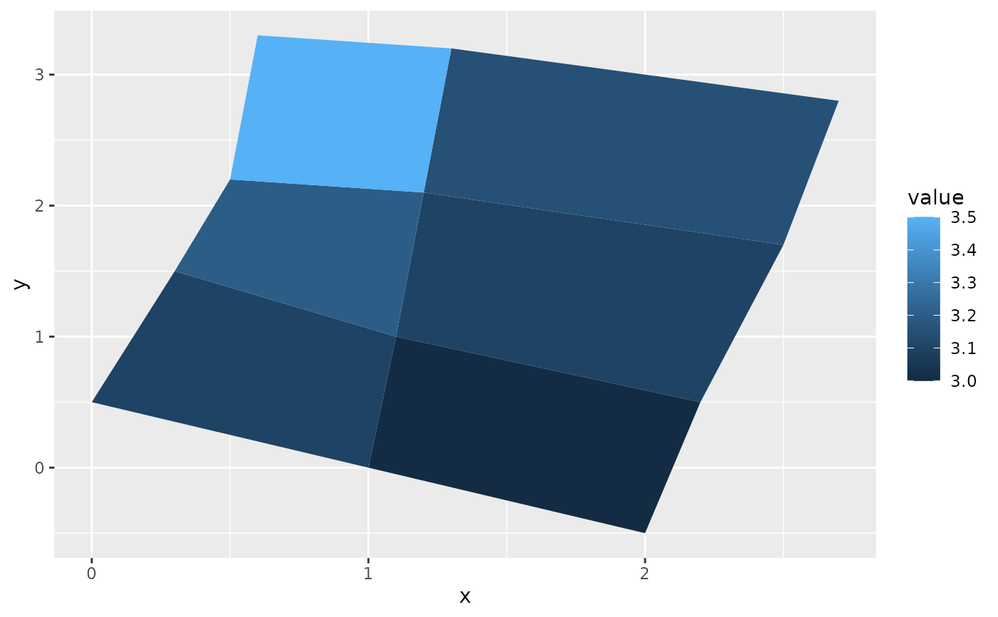
# When using geom_polygon, you will typically need two data frames:
# one contains the coordinates of each polygon (positions),  and the
# other the values associated with each polygon (values).  An id
# variable links the two together

ids <- factor(c("1.1", "2.1", "1.2", "2.2", "1.3", "2.3"))

values <- data.frame(
  id = ids,
  value = c(3, 3.1, 3.1, 3.2, 3.15, 3.5)
)

positions <- data.frame(
  id = rep(ids, each = 4),
  x = c(2, 1, 1.1, 2.2, 1, 0, 0.3, 1.1, 2.2, 1.1, 1.2, 2.5, 1.1, 0.3,
  0.5, 1.2, 2.5, 1.2, 1.3, 2.7, 1.2, 0.5, 0.6, 1.3),
  y = c(-0.5, 0, 1, 0.5, 0, 0.5, 1.5, 1, 0.5, 1, 2.1, 1.7, 1, 1.5,
  2.2, 2.1, 1.7, 2.1, 3.2, 2.8, 2.1, 2.2, 3.3, 3.2)
)

# Currently we need to manually merge the two together
datapoly <- merge(values, positions, by = c("id"))

p <- ggplot(datapoly, aes(x = x, y = y)) +
  geom_polygon(aes(fill = value, group = id))
p


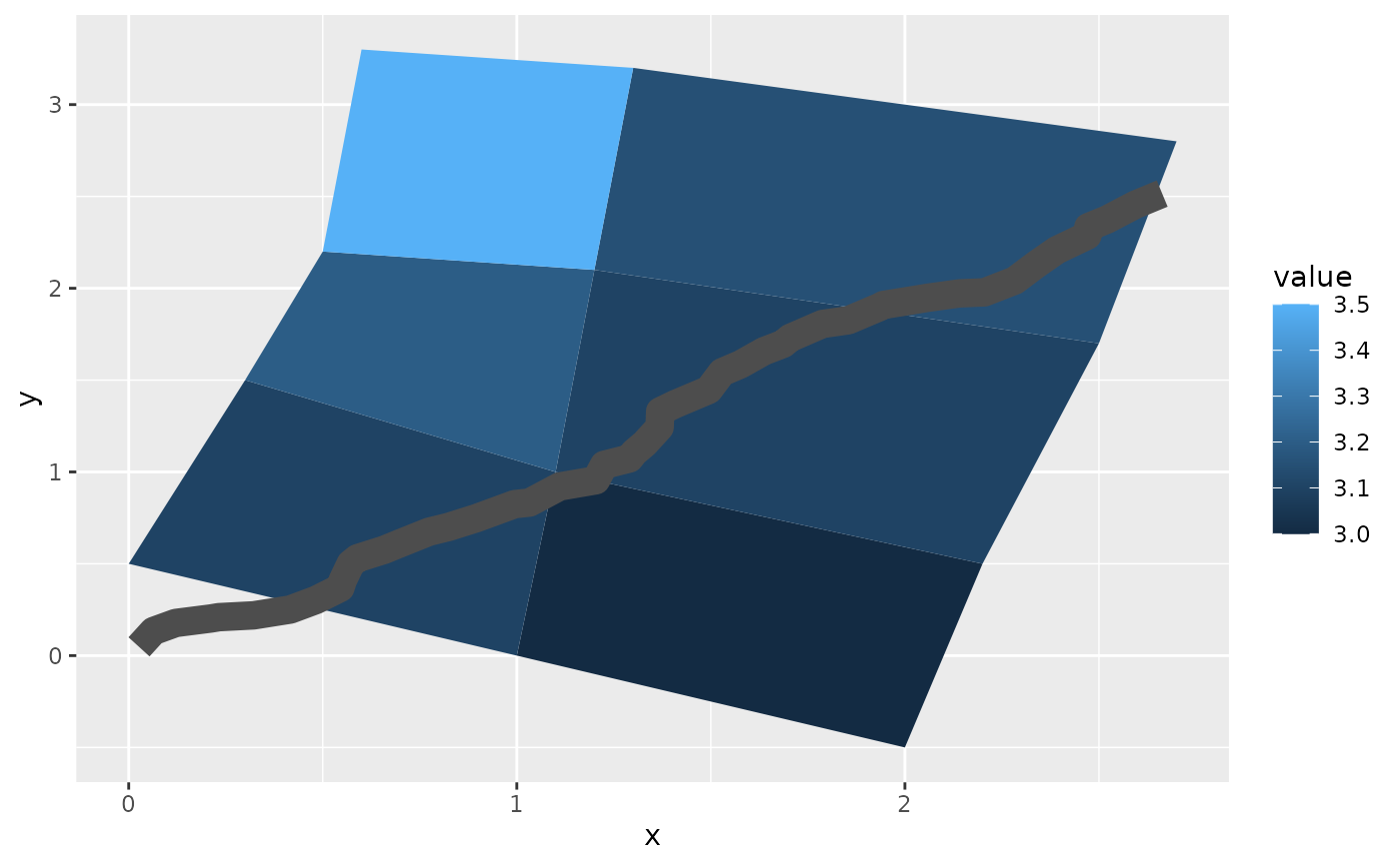
# Which seems like a lot of work, but then it's easy to add on
# other features in this coordinate system, e.g.:

set.seed(1)
stream <- data.frame(
  x = cumsum(runif(50, max = 0.1)),
  y = cumsum(runif(50,max = 0.1))
)

p + geom_line(data = stream, colour = "grey30", linewidth = 5)


# And if the positions are in longitude and latitude, you can use
# coord_map to produce different map projections.

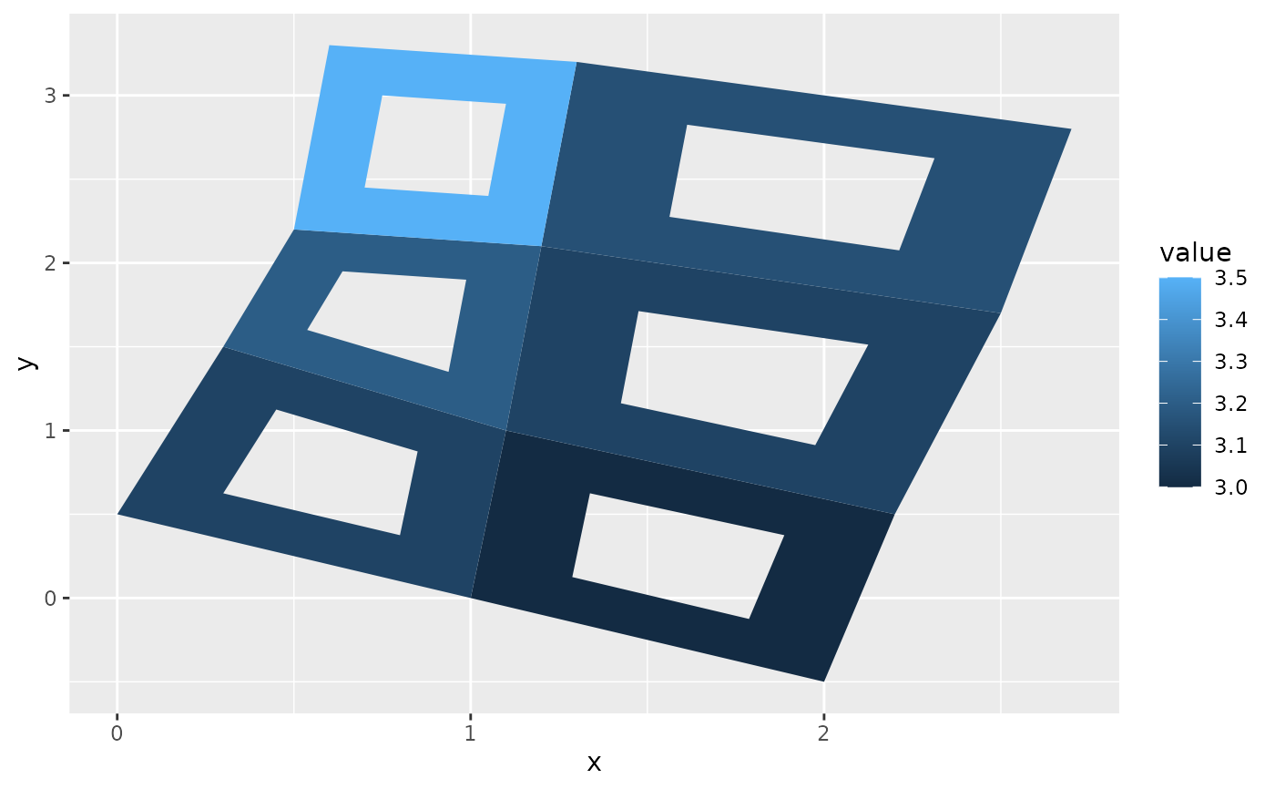
if (packageVersion("grid") >= "3.6") {
  # As of R version 3.6 geom_polygon() supports polygons with holes
  # Use the subgroup aesthetic to differentiate holes from the main polygon

  holes <- do.call(rbind, lapply(split(datapoly, datapoly$id), function(df) {
    df$x <- df$x + 0.5 * (mean(df$x) - df$x)
    df$y <- df$y + 0.5 * (mean(df$y) - df$y)
    df
  }))
  datapoly$subid <- 1L
  holes$subid <- 2L
  datapoly <- rbind(datapoly, holes)

  p <- ggplot(datapoly, aes(x = x, y = y)) +
    geom_polygon(aes(fill = value, group = id, subgroup = subid))
  p
}

Usage

Arguments

Aesthetics

See also

Examples